Multivariate Time Series Analysis
Multivariate time series (MTS) analysis involves the study of multiple related time series observed simultaneously. Unlike univariate analysis, which focuses on a single variable's past to predict its future, MTS explores the dependencies and interactions between different variables.
1. Motivation and Objectives
The primary goal is to shift from a scalar perspective to a Vector Process.
* Inter-relationships: Understanding how \(Y_{t}\) and \(X_{t}\) move together.
* Cross-relationships: Identifying lead-lag effects, such as how \(X_{t-2}\) might influence the current value of \(Y_{t}\).
* Improved Forecasting: Leveraging the information in auxiliary series (\(X_{t}\)) to produce more accurate forecasts for the target series (\(Y_{t}\)).
2. Domain Applications
MTS is essential in fields where variables are deeply interconnected:
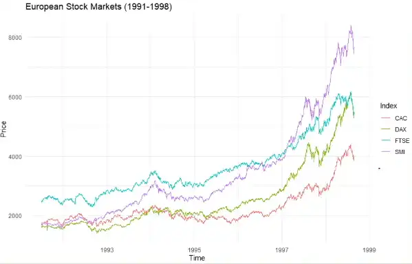
- Finance: Analyzing Bitcoin and Ethereum jointly to understand global market dynamics. Information in one market often spreads instantly to others, which is vital for portfolio management.
- Economics: Studying the simultaneous behaviors of inflation, interest rates, and GDP.
- Environmental Science: Modeling the joint impact of temperature, humidity, and wind speed on agricultural yields (e.g., wheat production).
- Public Health: Tracking the relationship between air pollution levels, traffic volume, and hospital admissions for respiratory issues.
3. Key Analytical Questions
When dealing with multiple series, we look beyond simple correlations:
* Causality: Is there a specific direction of influence (e.g., does \(X\) cause \(Y\))?
* Feedback Loops: Do the series influence each other bidirectionally?
* Impulse Response: How does a shock in one series (e.g., a sudden oil price hike) transfer to and affect the other series over time?
* Common Factors: Are there underlying "latent" variables causing disturbances across all observed series?
4. Mathematical Foundation: Matrix Algebra Refresher
To handle vector processes, we represent the systems using matrices. For an \(n \times n\) matrix \(A\):
- Eigenvalues (\(\lambda_{i}\)): The \(n\) roots of the characteristic equation \(|A - \lambda I_{n}| = 0\).
- Eigenvectors (\(q_{i}\)): Non-zero vectors satisfying \(Aq_{i} = \lambda_{i} q_{i}\).
- Diagonalization: If \(Q\) is a matrix of eigenvectors, then \(Q^{-1}AQ = \Lambda\), where \(\Lambda\) is the diagonal matrix of eigenvalues.
Important Properties:
* Determinant: \(|A| = \prod \lambda_{i}\) (Product of eigenvalues).
* Trace: \(trace(A) = \sum \lambda_{i}\) (Sum of eigenvalues).
* Matrix Powers: \(A^m = Q \Lambda^m Q^{-1}\) (Useful for calculating long-term stability in vector models).
5. Random Vector Properties
In MTS, we treat the observation at time \(t\) as a \(p \times 1\) random vector \(X_{t} = [X_{1t}, X_{2t}, \dots, X_{pt}]'\).
- Mean Vector: Contains the expected value \(E(X_{it})\) for each series.
- Variance-Covariance Matrix (\(\Sigma\)):
- Diagonal elements (\(\sigma_{ii}\)): The variance of each individual series.
- Off-diagonal elements (\(\sigma_{ij}\)): The covariance between series \(i\) and series \(j\).