Diagnostic Checking¶

Following Model Identification L16__Model Identification and Model Estimation L17__Model Estimation, the diagnostic stage is crucial to:
* Check the Goodness of Fit: Ensure the model accurately represents the underlying data structure.
* Validate Error Assumptions: Verify that the residuals (errors) satisfy the theoretical assumptions required for reliable forecasting.

1. Normality of Errors¶

We assume that errors follow a normal distribution ($e_{t} \sim \mathcal{N}(0, \sigma_{e}^{2})$). Several methods are used to verify this:

Visual Tools:
- Histogram: Plot the standardized residuals ($\frac{\hat{e}_{t}}{\sigma_{e}}$) to check for a bell-shaped curve.
- Normal Q-Q Plots: Plot theoretical quantiles (Standard Normal) against actual sample quantiles. A straight line indicates normality.
  
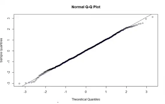
  Above: Normality holds true.
  
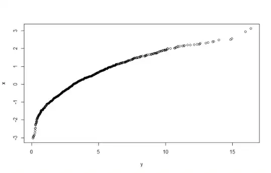
  Above: Normality does not hold.
Statistical Summaries: Using Tukey's "five-number summary," we check if the distribution matches normal parameters (Skewness $\approx 0$, Kurtosis $\approx 3$, Excess Kurtosis $\approx 0$). Note that small sample sizes may appear skewed even if drawn from a normal distribution.

Jarque-Bera (JB) Test¶

This test assesses whether the skewness ($\beta_{1}$) and excess kurtosis ($\hat{\beta}_{2} - 3$) are collectively zero.
$$JB = \dfrac{n}{6} \left[ \beta_{1}^{2} + \dfrac{(\hat{\beta}_{2}- 3)^{2}}{4}\right] \sim \chi_{2}^{2}$$
* $H_{0}$: Errors are normally distributed.
* $H_{a}$: Errors are not normally distributed.

Shapiro-Wilk Test¶

This test utilizes order statistics ($x_{(i)}$) and specific constants ($a_{i}$) to check for normality:
$$W = \dfrac{\left( \sum_{i=1}^n a_{i}x_{(i)} \right)^{2}}{\sum(x_{i}- \bar{x})^{2}}$$
* Decision Rule: Reject the null hypothesis of normality if the $W$ statistic is too small.

2. Detection of Serial Correlation¶

Serial Autocorrelation occurs when residuals are correlated with their own lagged values, suggesting that the model has not captured all the systematic information in the data.

ACF Plot of Residuals: If spikes in the ACF plot exceed confidence bands, serial correlation is present.

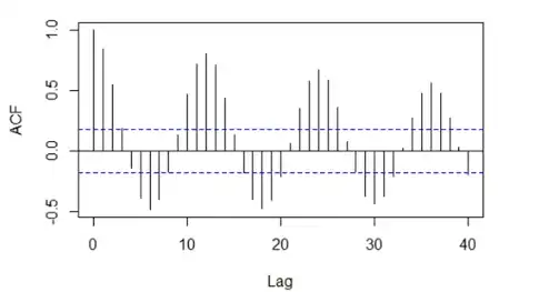
Above: Patterns in correlations indicate that current errors are related to past or future errors.

Box-Pierce Test¶

Used to test if a group of autocorrelations (up to lag $h$) is significantly different from zero.
* $H_{0}$: Residuals are independent (no correlation).
* Statistic: $Q_{BP} = n \sum_{k=1}^h \hat{\rho}_{k}^{2}$
* Action: If $Q_{BP} > \chi_{1-\alpha, h}^2$, reject $H_{0}$. You may need to add another lag to the AR or MA part of your model.

Ljung-Box Modified Test¶

A more robust version of the Box-Pierce test, modified in 1978 to perform better with smaller sample sizes.
$$Q_{LB} = n^{2} \sum_{k=1}^h \dfrac{\hat{\rho}_{k}^{2}}{n-k}$$
* The setup remains the same as the Box-Pierce test, but the formula accounts for the sample size ($n$) and lag ($k$) more precisely in the denominator.