Examples and Goals of Time Series Data
1. Why is Time Series (TS) Important?
Time Series analysis allows us to look beyond static data points to understand the temporal dynamics of a process. Its importance lies in:
- Understanding Patterns: It helps identify underlying trends and patterns, which eventually allows us to estimate how data will move in the future.
- Predictive Power: We can predict the likelihood of future events (e.g., determining if a stock price is likely to go up or down).
- Statistical Inference: It enables us to make inferences about the probability models governing a series, including determining confidence intervals and estimating model parameters.
2. Time Series Notation
To represent time series mathematically, we use specific notation to track observations over intervals:
- Sequence: \(X_{t}, X_{t+h}, \dots\) where \(t\) is the time point of the first observation and \(h\) is the time elapsed between observations.
- Sampling Frequency: This is defined as \(\dfrac{1}{h}\), representing how often observations are recorded.
- Dependency: The order of observations is critical because observations in a time series are typically dependent on one another.
- Example: In a series \(X_{t}, X_{t+2}, \dots\), the gap \(h = 2\). Therefore, the sampling frequency is \(1/2\) (e.g., half an observation per day).
3. Practical Examples of Time Series Data
The behavior of a series is often categorized by its trend (long-term direction) and seasonality (repetitive patterns).
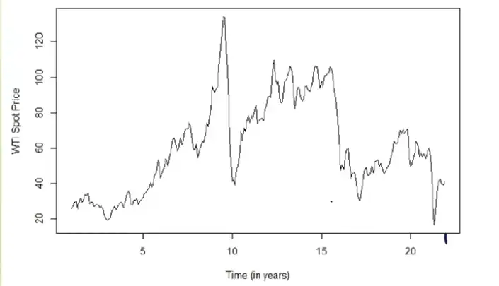
- Example 1: Carbon-dioxide Levels: Exhibits a clear upward trend with distinct repetitions due to underlying seasonality. * Example 2: Oil Spot Price ($/barrel): Typically shows no overall trend and no apparent seasonality, often appearing highly stochastic.
 * Example 3: SGST (State GST) Revenues of India: Characterized by a mild upward trend as economic activity grows over time.
 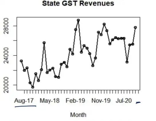 * Example 4: Delhi Air Quality (2017-2020): Shows no overall trend, though mild trends may appear in small batches. Seasonality is highly present (e.g., winter peaks), usually observed on a monthly time scale.
 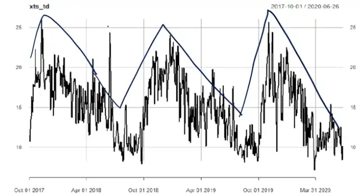 * Example 5: Quarterly Sugarcane Prices: Observed on a quarterly time scale, specifically chosen based on the agricultural and economic purpose of the study.
 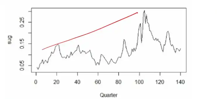 * Example 6: Indian Population: A classic example of a long-term trend. * Example 7: International Airline Data: Represents a non-stationary seasonal time series. It features an upward trend and clear seasonality (low in winter, high in summer).
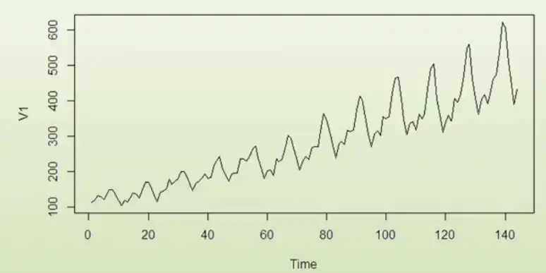
4. Choosing Time Scales and Series Length
Selecting the appropriate interval is crucial for meaningful analysis:
* Time Scale Selection: When analyzing data like stocks (available at ticker level), consider the scale of required forecasts and the level of noise (random fluctuations). For example, to forecast next-day sales, daily data is sufficient; minute-by-minute data would introduce unnecessary noise.
* Long vs. Short Time Series:
* Long Series: Contains many observations (e.g., weekly interest rates or daily stock prices over 5 years).
* Short Series: Contains limited observations (e.g., daily stock prices over a single month, yielding only ~22 observations).
5. Goals of Time Series Analysis
The ultimate objectives of TS analysis are generally two-fold:
1. Explanatory: To understand the underlying stochastic mechanisms and probability models that give rise to new data points.
2. Predictive: To use that understanding and the historical data of the series to accurately predict future values.