Non-stationary Time Series¶

In real-world applications, time series data usually exhibits Trend, Seasonality, or Cyclicality, making it inherently non-stationary. To analyze such data, we must transform it into a stationary series using mathematical operators.

1. Mathematical Operators¶

Two primary operators are used to manipulate and stabilize time series data:

Backshift Operator ($B$): Shifts the observation back by $d$ time units.
$$B^dY_{t} = Y_{t-d}$$
Differencing Operator ($\nabla$): A technique popularized by Box & Jenkins to remove non-stationary components.
- First Difference: $\nabla Y_{t} = Y_{t} - Y_{t-1} = (1-B)Y_{t}$
- Second Difference: $\nabla^2 Y_{t} = \nabla(\nabla Y_{t}) = Y_{t} - 2Y_{t-1} + Y_{t-2}$
- Lag $d$ Difference: $\nabla_{d}Y_{t} = Y_{t} - Y_{t-d}$ (Used primarily for removing seasonality).

2. Eliminating Trends through Differencing¶

Example 1: Linear Trend¶

Consider a model with a linear trend: $Y_{t} = bt + S_{t}$. It is non-stationary because the mean is time-dependent. Applying a first difference:
$$\nabla Y_{t} = bt + S_{t} - (b(t-1) + S_{t-1}) = S_{t} + b - S_{t-1}$$
The result is now stationary as the time-dependent term $t$ is eliminated.

Example 2: Quadratic Trend¶

For a stronger trend like $Y_{t} = bt^{2} + S_{t}$, a single differencing is insufficient. We apply the second difference operator:
$$W_{t} = \nabla^{2}Y_{t} = Y_{t} - 2Y_{t-1} + Y_{t-2}$$
This eventually simplifies to:
$$W_{t} = 2b + S_{t} - 2S_{t-1} + S_{t-2}$$
The quadratic growth is neutralized, resulting in a stationary process.

3. Random Walk as a Non-Stationary Process¶

The Random Walk model is $Y_{t} = Y_{t-1} + e_{t}$. If viewed as an $AR(1)$ process:
$$Y_{t} = c + \phi_{1} Y_{t-1} + e_{t}$$
Here, $c=0$ and $\phi_{1} = 1$. Recall that for an $AR(1)$ process to be stationary, we require $|\phi_{1}| < 1$. Since $\phi_{1} = 1$ (often called a Unit Root), the random walk is fundamentally non-stationary.

4. Seasonal Models and Decomposition¶

In the classical decomposition model, a series is expressed as:
$$Y_{t} = m_{t} + s_{t} + S_{t}$$
* $m_{t}:$ Trend component.
* $s_{t}:$ Seasonal component with period $d$.
* $S_{t}:$ Stationary process (noise).

Transformation Rules

Lag $d$ difference ($\nabla_d$): Removes seasonality of period $d$.
Lag 1 difference ($\nabla$): Applied multiple times, it removes the trend aspect of the series.

5. The $ARIMA(p,d,q)$ Process¶

The AutoRegressive Integrated Moving Average (ARIMA) model is used when a series becomes stationary after being differenced $d$ times.

Definition:
If $W_{t} = \nabla^d Y_{t} = (1-B)^d Y_{t}$ is a stationary $ARMA(p,q)$ process, then the original series $Y_t$ is an $ARIMA(p,d,q)$ process.

p: Order of the Autoregressive part.
d: Degree of differencing involved.
q: Order of the Moving Average part.

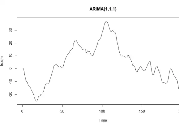
Example: An $ARIMA(1,1,1)$ with $\phi_{1} = 0.7$ and $\theta_{1} = 0.2$ implies the first difference of the data follows an $ARMA(1,1)$ structure.