Verrall: Expert Opinion
Study Strategy
Checklist
- Know why an actuary may want to intervene in the parameter selections and which experts may be consulted for expert opinions
- Know the advantages of using the Bayesian model for inserting expert opinion
- Be able to list the simplifying assumptions made by Verrall
- Be able to calculate the expected value and variance for the different distributions:
- Mack model
- Over-dispersed Poisson
- Over-dispersed negative binomial
- Normal
- Be able to list advantages and disadvantages of the different distributions
- Know the basics of MCMC methods, especially the impact of the standard deviation selection for the prior distribution
- Know what prediction error is and the different parts of prediction error
- Know why Bayesian methods are superior when it comes to calculating the prediction error
- Know the impact of the standard deviation selection on the prediction error
- Know how to adjust LDFs in Bayesian models for expert opinion:
- Select separate LDFs for each row
- Use only the most recent \(N\) diagonals
- Know how to adjust ultimate losses in Bayesian models for expert opinion:
- Recognize the BF formula
- Be able to calculate the BF estimates of incremental losses
- Be able to explain how the BF formula is a credibility weighting of the chain ladder and BF methods and point out the chain ladder and BF parts of the formula
- Be able to explain the impact of \(\beta\) on the variance and \(Z_{ij}\)
- Understand how to use row parameters to calculate incremental losses
- Know why we would want to use row parameters
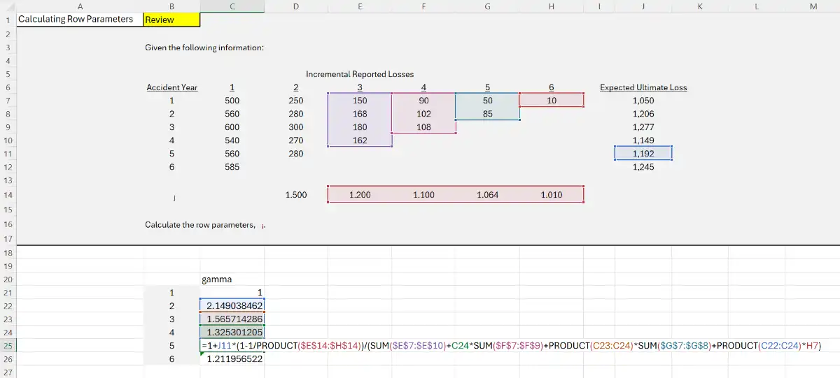
- Be able to calculate the row parameters, \(\gamma_i\)
My Notes
-
Actuarial judgement → Intervene in parameter selection. Why? Reasons include
- Internal policy changes → change in payment patterns
- Legislative changes → change in potential loss development
-
When can we incorporate expert opinion?
- Residuals in ODPB? → NO! Invalidates model assumptions
- CL → adjust LDFs → How does it affect/change the variance of losses? So variance is no longer valid
- \(\implies\) Use a Bayesian model. Why?
- Allow incorporation naturally, without violation
- Easy
- Gives full distribution (not just mean/variance) of losses
Notation and Assumptions
- \(C_{ij}\) → Incremental
- \(D_{ij}\) → Cumulative
- \(\lambda_{j}\) → LDF
- \(M_{i}\) → expected losses = \(\text{ELR} \times\text{Premium}\)
-
\(y_{i}\) → incremental \% reported
-
Simplifying assumptions about data
- Triangular and,
- Fully Developed → No tail factors needed
Loss Distributions
- Mack = Chain Ladder + Variance info
- GLM1
- ODP
- \(E(C_{ij}) =m_{ij}\) and \(\ln[m_{ij}]=\alpha_{i} + \beta_{i}\)
- \(Var(C_{ij}) = \phi m_{ij}\)
- Con → negative incremental values become a problem (log of negative number doesn't exist)
- ODNB
- Same predictive distribution as ODP (reserve estimates and moments are identical)
- But Correction to CL is apparent in the mean: You look at the mean formula, and it screams "Chain Ladder"
- \(E[D_{ij}|D_{i,j-1}, \lambda_{j}, \phi] = \lambda_{j}D_{i,j-1}\)
- \(Var[D_{ij}|D_{i,j-1}, \lambda_{j},\phi]=\phi(\lambda_{j}-1)\lambda_{j}D_{i,j-1}\)
- Pro → negative increments are not a problem
- Con → if sum of column is negative \(\lambda_{j}\lt 1\) → variance negative
- Same predictive distribution as ODP (reserve estimates and moments are identical)
- Normal
- \(E[D_{ij}|D_{i,j-1},\lambda_{j},\phi] = \lambda_{j}D_{i,j-1}\)
- \(Var[D_{ij}|D_{i,j-1},\lambda_{j},\phi]= \phi D_{i,j-1}\)
- Pro → Can handle negative column sums too!
- ODP
Markov Chain Monte Carlo (MCMC) methods
The wider priorōs we select the more the posterior distribution will correspond to the data (i.e. chain ladder results). The narrower our priors are, the more the posterior will be in line with our expert opinion and will disregard the data.
- MCMC methods simulates one parameter at a time (conditional on values of other params) → creating a Markov chain where each param is considered in turn (instead of all at once)
- Select prior for each parameter. Conditional distribution3. Combine these distributions → Posterior (to estimate future losses). Posterior is in between the prior distribution and the conditional distribution (data) spectrum.
- Wide prior → SD is very large \(\implies\) Posterior → conditional distribution side of spectrum.
- Narrow prior → SD small \(\implies\) Posterior → close to mean selected for prior distribution side of spectrum
- SD \(\uparrow\) \(\implies\) closer to the conditional. SD \(\downarrow\) \(\implies\) closer to the prior mean
Prediction Error
or
Bayesian \(\gg\) Non-Bayesian
- Non-Bayesian methods only calculate estimation variance (SE\(^{2}\))
- Calculation of process variance is done separate and is complicated.
- Bootstrap process → straightforward method to estimate process variance
Also, it produces the full distribution, including prediction error when run.
Large Standard deviation (wide priors ) \(\implies\) low confidence in parameters \(\implies\) larger prediction error.
Adjusting Bayesian Models with Expert Opinion
- Insert expert opinion by selecting mean and SD of prior distribution
- If no opinion → Wide prior (any mean)
- If yes → set mean to our opinion and SD to how sure we are about it (more sure \(\implies\) smaller SD)
- Opinion can be from a reserving actuary, or from claims leadership or underwriter (whoever has the expertise)
The Idea is important
The adjustments discussed are mere examples as to how expert opinion can be incorporated. The idea can be extended to other use cases / situations too!
Adjustment Type 1: Selecting Separate LDFs for each row
- Standard CL → Same Dev factors for each row (varying by column) \(\lambda_{j}\)
- But sometimes we need \(\lambda_{ij}\) that varies by both
- Use negative binomial distribution
- Specify priors for LDFs
- Lean towards CL LDFs → Large SD
- Predetermined LDF → Small SD
Opinion: AY 4, 5, and 6 for Dev (2,3) should be 1.15
The rest of the groups have mean 1 and infinite variance.
Adjustment Type 2: Only Use the Most recent \(N\) diagonals
- Divide 6x6 triangle (full) data into two groups:
- \(\lambda_{ij}= \lambda_{j}\) for \(i = 7-j, 6-j, 5-j\)
- \(\lambda_{ij} = \lambda_{j}^*\) for \(i= 1,2,\dots,4-j\)
| 1 | 2 | 3 | 4 | 5 | 6 | |
|---|---|---|---|---|---|---|
| 1 | * | * | * | \(\lambda_{4}\) | \(\lambda_{5}\) | \(\lambda_{6}\) |
| 2 | * | * | \(\lambda_{3}\) | \(\lambda_{4}\) | \(\lambda_{5}\) | |
| 3 | * | \(\lambda_{2}\) | \(\lambda_{3}\) | \(\lambda_{4}\) | ||
| 4 | \(\lambda_{1}\) | \(\lambda_{2}\) | \(\lambda_{3}\) | |||
| 5 | \(\lambda_{1}\) | \(\lambda_{2}\) | ||||
| 6 | \(\lambda_{1}\) |
- Give each set \(\lambda_{j}^*\) and \(\lambda_{j}\) → large variances so that they are estimated from data.
- Then just use \(\lambda_{j}\) for future loss estimates (and not \(\lambda_{j}^*\))
A Bayesian Model for Bornhuetter-Ferguson
- Incorporate expert opinion in ultimate loss estimate (not LDFs)
- Expected loss in each row: \(M_{i}\) → Gamma distribution
Set \(\alpha\) and \(\beta\) in such a way that the desired mean and variance are obtained. Decrease \(\beta\) to increase variance and adjust \(\alpha\) to keep the mean fixed \(M_{i} = 500\). So, the more we are sure about \(M\), the larger the \(\beta\) should be.
- It's actually Benktander (cred weighting between B-F and Chain Ladder)
- The credibility weighs the incremental loss derived (by doing \(\times (LDF-1)\)) from Actual losses to date (\(D_{i,j-1}\)) and Expected Losses to date (\(=M \times\text{\%reported}\))
where,
- \(Z_{ij}\) → credibility factor. Cum % reported is the numerator.
- \((\lambda_{j}-1)D_{i,j-1}\) → chain ladder estimate of incremental losses
- \((\lambda_{j} - 1) M_{i} \dfrac{1}{\lambda_{j}\lambda_{j+1}\dots\lambda_{n}}\) → B-F estimate of incremental losses2
Work out an example
- \(\alpha = 250\), \(\beta = 0.011\), \(\phi = 9.13\)
- \(\lambda_{j} = [1.5, 1.2, 1.1, 1.0]\)
- Compute BF estimate of incremental loss from 12 to 24 month maturity
- More the \(\beta\), more confident we have in our a priori. We should adjust \(\alpha\) such that the expected value \(M_{i}\) remains the same.
Estimating Row Parameters
- Chain ladder estimates can be computed using row parameters, called \(\gamma_{i}\), rather than traditional LDFs.
- Expected incremental losses are given by:
or
Why use row parameters?
- To create a fully stochastic model.
- We first estimate column parameters (LDFs)
- Use those to estimate row parameters
How to calculate \(\gamma_{i}\)?
Given,
- \(\lambda_{j}\) → development factors
- \(x_{i}\) → Expected ultimate losses
And for \(i=3,\dots,n\)
Don't memorize
This is a daunting formula, you might make mistakes while memorizing the indices.
So instead, just try to understand the pattern of these calculations.
Expert Opinion incorporated
- \(x_{i}\) is our prior distribution for our MCMC model
- The \(\gamma\) will be our conditional distribution3
- Smaller the SD → closer estimated losses would be to \(x_{i}\)
FAQs
"ODNB has the same predictive distribution as ODP, with the advantage that the connection to chain-ladder is apparent in the mean". So does it mean that ODP doesn't have a connection with Chain Ladder? (This contradicts Taylor)
It feels like a contradiction because, as correctly noted from Taylor’s paper, the Over-Dispersed Poisson (ODP) is the "poster child" for the GLM equivalent of the Chain-Ladder.
Verrall isn't saying ODP isn't connected to Chain-Ladder. Instead, he is making a point about parameterization and how "obvious" the math looks in a Bayesian framework.
1. The ODP and Chain-Ladder Connection
You are 100% correct about Taylor. In a frequentist GLM, the ODP model with a logarithmic link function and row/column parameters (\(\alpha_i\) and \(\beta_j\)) yields the exact same reserve estimates as the Mack Chain-Ladder.
-
The ODP Mean Structure: \(E[Y_{ij}] = \alpha_i \beta_j\)
-
While the results match Chain-Ladder, the parameters (\(\alpha, \beta\)) don't look like "development factors" (\(f_j\)) on their own. You have to do a bit of algebraic gymnastics to see how the column parameters relate to the \(1.25\) or \(1.10\) factors you are used to.
2. Why Verrall Says ODNB is "More Apparent"
In Verrall’s Bayesian ODNB model, he sets up the mean structure differently. He parameterizes the model such that the development factors themselves are the parameters you are estimating.
-
The ODNB Mean Structure: \(E[Y_{ij}] = C_{i, j-1} (\lambda_j - 1)\)
-
Here, \(C_{i, j-1}\) is the cumulative loss at the previous period.
-
\(\lambda_j\) is the Chain-Ladder development factor.
-
In this setup, the "link" to Chain-Ladder is sitting right there in the formula for the mean. You don't have to derive it; the model is explicitly built using the logic: "Today's incremental loss is yesterday's total multiplied by a factor."
3. The Predictive Distribution Point
When Verrall says they have the same predictive distribution, he means that if you set them up with the same priors and mean structures, they will give you the same range of possible outcomes (the same "error bars").
The ODNB is often preferred in Bayesian software (like WinBUGS or Stan) because:
-
Over-dispersion: The Negative Binomial naturally handles cases where the variance is greater than the mean without needing the manual "phi" (\(\phi\)) adjustment required by the ODP.
-
Interpretation: It is easier for an actuary to set a "prior" on a development factor (e.g., "I think the 12-to-24 month factor is around 1.5") than it is to set a prior on an abstract \(\beta_j\) parameter in a Poisson log-linear model.
Summary
-
Taylor is right: ODP connects to Chain-Ladder via the resulting estimates.
-
Verrall is right: ODNB is "more apparent" because the Chain-Ladder factors (\(\lambda_j\)) are the actual variables in the equation for the mean, making it more intuitive for Bayesian modeling.