Venter: Validate LDF Assumptions

Study Strategy

• Tests are easy, just study them and treat them as an extension to what we did in the last paper (Mack-Chainladder).
  • Only thing I'd suggest is to not spend too much time on the #Superiority of emergence pattern test ( 1) now and get to it only when you start practicing

Checklist

1. Know that under Mack's assumptions, the chain ladder method is the minimum variance unbiased linear estimator of future emergence
2. Be able to perform the different assumption tests, know if the data passes or fails the test, and know what assumption it's testing
   • Significance test
   • Superiority of emergence pattern test
   • Linearity test
   • Stability test
   • Correlation test
   • Diagonal dummy regression test
3. Be able to calculate \(f(d)\) and \(h(w)\) for the parameterized BF or Cape Cod methods for constant variance or variance proportional to loss
4. Understand how to calculate the number of parameters for a BF-CC emergence pattern
5. Be able to calculate expected ultimate losses using the additive chain ladder method

My Notes

Remember

• Venter always uses incremental development factors so \(f(d)\) will not be \(\gt 1\) in general.
• Plot \(Y\) vs \(X\)

Assumptions

1. Expected value of incremental losses in the next period \(\propto\) Losses to date
   • E(incremental losses) in then next period is equal to cumulative losses to date times a factor that depends on age.
2. Losses are independent across AYs
3. The variance of the next incremental losses \(= f(\)cumulative losses to date\()\)
   • Var(incremental losses) in then next period is proportional to cumulative losses to date by a factor that depends on age.

Tests

Test (Assumption #)	What to do?	What to check?	If failing?
#Significance test ( 1)	Regress	check if \(a\) and \(b\) are significant?	Use #Additive Chain Ladder (if \(b\) significant)
#Superiority of emergence pattern test ( 1)	Use Adj. SSE (or info criteria)	compare "prop emergence" to other patterns.
#Linearity test ( 1)	Plot residual vs loss	No pattern (random scatter) , constant variance
#Stability test ( 1)	Plot LDF vs time	Relatively flat (5yr), no trends else unstable	Unstable → Give more weight to recent years
#Correlation test ( 2)	\(T_{n-2} = r\sqrt{ \dfrac{n-2}{1-r^{2}} }\)	\(H_{0}:\text{No Correlation}\)
#Diagonal dummy regression test ( 2)	Regress with dummy for diagonals \(d_{j}\).	If dummies are significant → CY effect exist.

Significance test (#1)

Test

Are the loss dev factors (statistically) significant?

• constant = \(a\), factor = \(b\)
• Value of \(x > 2\times SD(x)\) \(\implies x\) is significant
• To prefer Chainladder: \(b\) should be significant but \(a\) should NOT be significant.

• What happens if \(a\) is significant but \(b\) is not? → Use #Additive Chain Ladder

Superiority of emergence pattern test (#1)

Test

Is proportional emergence superior to other emergence patterns?

• Calculate Adjusted SSE \(\dfrac{SSE}{(n-p)^{2}}\) for different models.
  or AIC = \(SSE \times e^{ 2p/n }\) or BIC = \(SSE \times n^{p/n}\)

• Select the model with the lowest value.

Use incremental losses.

• Models to compare against
  1. Linear with constant \(y = b +ax\)
  2. Factor times parameter: \(y = f(d)h(w)\)

Linearity test (#1)

Test

Test for linearity (residuals vs losses to date should be random)

• Residuals should be random about zero (no patterns)
  • Should scatter randomly around zero
  • Magnitude should not change with time

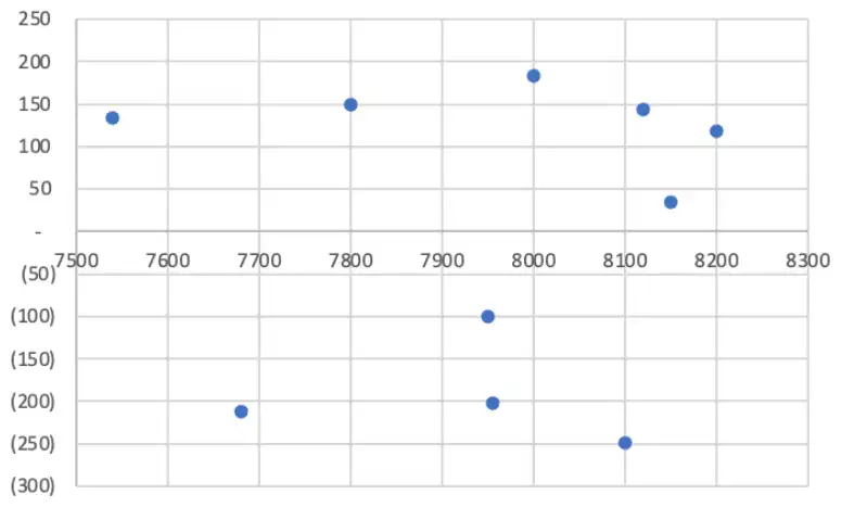
Here \(\downarrow\) we se a clear pattern in residuals \(\implies\) Fails the test, thus non-linear.

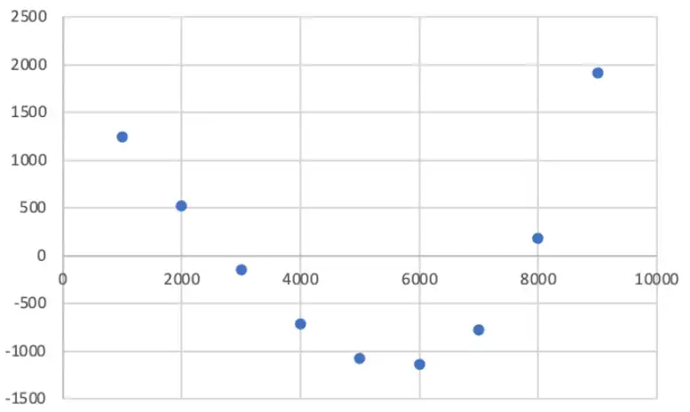
But here \(\downarrow\) the residuals look much more random \(\implies\) Passes linearity test

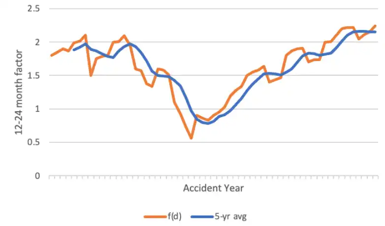
Stability test (#1)

Test

Are the development factors stable over time?

• LDF plotted against time
• 5-year average line should be relatively flat \(\implies\) factors are stable
• Trends in the LDFs \(\implies\) unstable,
  • try giving more weight to recent years

In this example \(\downarrow\) , the factors are not stable (the blue line is not flat)!

Other tests

1. Plot residuals against time (residuals should be random around 0)
2. Use a state-space model¹

Fix for a failing test?

• Use a weighted average with more weight on the more recent years
• Use a 5-year weighted average
• Use a 5-year simple average
• Use a 5-year ex hi/lo average
• Exclude the accident years where the age-to-age factors are lower
• Fit a curve to the age to age factors
• Use expert opinion to select the age-to-age factor
• Use industry data to select the age-to-age factor
• Adjust the triangle through the Berquist Sherman method
• Use the state-space model

Correlation test (#2)

Test

Correlation T-test to see if AY's are correlated. (unlike Spearman's rank test for development period correlation)

• Calculate \(f(w,d)\) - incremental factor
• Calculate sample correlation \(r\) (=correl)
• Calculate \(T = r\sqrt{ \dfrac{n-2}{1-r^{2}} }\)
• Test the hypothesis

Diagonal dummy regression test (#2)

Test

Diagonal dummy regression test

• \(y = \beta_{0} + \beta_{1}x + \beta_{2}d_{1} + \beta_{3}d_{2}\dots\)
• \(d_{j}=\begin{cases} 1, & \text{loss is in the j-th diagonal} \\ 0, & \text{otherwise}\end{cases}\)
• If any of the dummies, \(d_{j}\) are significant \(\implies\) Calendar year effects exist & Chain Ladder is inappropriate

Parameterized BF Method

• The method is simple, just iteratively calculate \(f(d)\) and \(h(w)\), with the initial values (of \(f\) or \(h\) given).
• There are two variance assumptions, according to which the iterative equations change.

Var Assumption	Constant	Proportional
\(h(w)=\)	\(\dfrac{\sum{q}\times{f}}{\sum{f\times f}}\)	\(\dfrac{\sum{q^2} \div {f}}{\sum{f^2 \div f}}\)
\(f(h)=\)	\(\dfrac{\sum{q}\times{h}}{\sum{h\times h}}\)	\(\dfrac{\sum{q^2} \div {h}}{\sum{h^2 \div h}}\)

Careful

We need to use incremental values \(q(w,d)\) for this process.

Cape Cod Parameters

There are too many parameters in Parameterized BF, we can improve this situation by using Cape Cod Parameters, i.e. ONLY ONE \(h(w)\) for all AY's \(w\). For this, we use the same iterative formula as mentioned above, but for \(h(w)\) instead of summing row-wise, we will use all rows and columns of data to get A SINGLE \(h(w)\) value.

BF-CC Emergence Pattern

Another way to get fewer parameters is to group AYs (\(h(w)\)) and development periods (\(f(d)\)) which aren't significantly different.

Number of parameters

\(p\), the number of parameters should only include those parameters which are required for estimation. For example, we can skip the \(f(d)\) parameter for 0-12 period. Because all of the losses in the 0-12 period are known, and thus it won't be useful calculating \(f(1)\). If all the losses for 12-24 period were also known (not a proper triangle that way but still, for the sake of explanation)… then we would select number of parameters excluding \(f(d)\) parameters for 0-12 and 12-24, as they don't require any estimation.

Additive Chain Ladder

• When constant terms are significant in #Significance test ( 1) but factor values are not!
• Gives the same fit accuracy as Cape Cod Method
• Additive (and BF and CC) allows for a bad year to be in just a few development periods. But traditional chain ladder amplifies the effect of the bad losses and carries them through all development periods.

NOTATION: Instead of factors \(f(d)\), find average development \(g(d)\) → Average of increments.

---

1. State-space model is a formal statistical model that measures the amount of instability around the current mean and the instability in the mean itself over time. ↩

Comments