Teng & Perkins: Retro Rating & Asset Premiums

Study Strategy¶

Checklist¶

My Notes¶

Retro adjustments
- First at 18 months of losses (+9 lag = 27 months of booked premium)
- Subsequent +12 to both (refer to table below)

Retro adj.	Losses a/o	Booked Prem a/o
1	18 months	27 months	Blue
2	30 months	39 months	Yellow
3	42 months	51 months	Green
4	56 months	Not yet reflected	N/A

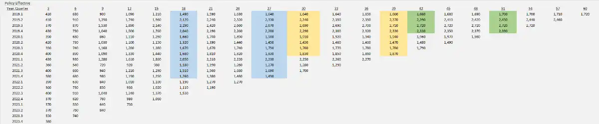
Note that in our calculations, the retro premiums should have reflected in the book. Thus we don't consider 18 month losses from 2022.2, 2022.3 & 2022.4 even though the retro adjustment has already been done. This is due to the lag.

Retrospectively Rated Insurance¶

After the policy expires → premium is set to reflect actual experience (premium adjusts up or down as losses develop)

Features
1. Even with no losses insured pays minimum premium
2. There has to be a maximum premium (else no point of buying insurance)¹
3. There is a per accident loss limit that caps the amount of individual loss that can contribute to the additional premium being collected
Benefits
1. Good experience \(\implies\) Premium refunds.
  - This purchase is attractive for insureds with good loss control and management procedures
  - Insurer can attract good consumers this way
2. Policyholders benefit by paying premiums gradually (instead of fully up-front). This way, they hold on to cash for longer \(\implies\) possible investment income.
3. Insurer benefits → risk due to inflation, rate regulations, increasing claim frequency², and lawsuits → shift to the insured \(\implies\) improves availability of insurance.

Retrospective Premium¶

\[ R = (b + CA)T \]

where
- \(CA:\) \(\text{Loss Conversion Factor}\times\text{Capped incurred Loss}\)
  - to cover incurred losses (capped at per accident limit) and,
  - expense → LAE (represented by \(C\), loss conversion factor), taxes (factor \(T\) multiplied to it) and other state assessments.
- \(b:\) basic premium includes \(= e - (C-1)E[A] + CI\)
  - expense provision (company expenses)
    - UW
    - acquisition
  - insurance charge (min and max)
    - insured needs protection against large losses \(\implies\) max
      - losses \(\gt\) max → insured benefits, insurer loses
    - insurer needs to collect enough premium (cover expenses, bit of losses) \(\implies\) min
      - losses \(\lt\) min → insurer gains, other loses
    - IC \(=E(\text{Loss due to max}) - E(\text{Gain due to min})\)
  - excess loss charge → accounting for risk of losses exceeding per-accident loss limit.

PDLD Ratio¶

Disclaimer

These methods are meant to be applied to an entire (or large segment of) book of business, rather than individual policies

Rating Parameter¶

Rating Parameter	Name	Description
\(P_{n}\)	Premium at \(n\)-th retro adjustment
\(BP\)	Basic premium
\(SP\)	Standard Premium
\(\dfrac{BP}{SP}\)	Basic Premium factor
\(L_{n}\)	Total developed at \(n\)-th retro adjustment
\(CL_{n}\)	Capped loss at \(n\)-th adjustment	Any loss contributing to additional premiums
\(LCR_{n}\)	\(\dfrac{CL_{n}}{L_{n}}\) = Loss capping ratio (% contributing to additional premium)	- \(\downarrow\) as data matures - If loss data already capped, \(L_{n} = CL_{n}\) and \(LCR_{n}=1\) - Otherwise, the ratio needs to be estimated - LCR = 0.9 \(\implies\) 1-0.9 = 10% of losses are eliminated by max, min and per
\(LCF\)	Loss Conversion Factor	loss-related expenses
\(TM\)	Tax Multiplier	premium taxes and other state assesments

\[ P_{n} = [BP + (CL_{n}\times LCF)] \times TM \]

which is same as

\[ R = (b + AC)T = (b + CA)T \]

\[ L_{n} = SP \times E[\text{Loss Ratio}] \times \% \text{Loss Emerged} \]

Deriving this formula makes more sense, just remember the basic identities, and the fact that you have to break \(L_{n}\) and also use \(LCR_{n} = \dfrac{CL_{n}}{L_{n}}\).

\[ PDLD_{1} = \dfrac{P_{1}}{L_{1}} = \left(\dfrac{BP}{SP} \times \dfrac{TM}{ELR \times \%Loss_{1}}\right) + [LCR_{1} \times LCF \times TM] \]

There are two parts in this formula:

\(\left(\dfrac{BP}{SP} \times \dfrac{TM}{ELR \times \%Loss_{1}}\right)\) → Charged even without loss, cost to write and service the policy (unrepeated in subsequent adjustments)
\([LCR_{1} \times LCF \times TM]\) → cost of the policy for any reported losses (will be adjusted again)

And then,

For \(PDLD_{2} = \dfrac{P_{2}-P_{1}}{L_{2}-L_{1}}\)
- Eventually instead of \(LCR_{1}\) write the incremental Loss Capping Ratio, \(\dfrac{CL_{2}-CL_{1}}{L_{2} - L_{1}}\) in the (2) part
Pros:
- change to rating params can be accounted for (good for currently written policies)
- PDLDs are more stable than #Empirical method
Cons
- rating parameters (LDF) cannot be average across segments (to avoid bias)
  - thus have to retrospectively test PDLD ratios (actual vs expected)

Empirical¶

Don't use ultimate losses because future actual loss development will be accounted for in future premium adjustments.

Aggregate by Policy effective Quarter³
Say the first adjustment is done at 18 months, there is a lag in processing and recording adjusted premiums → for them to be booked it will take some more months after the adjustment has been made. (use Lag = 9 months unless stated otherwise)
So we have to associate losses at 18 months with premiums booked at 27 months.
- Second adjustment is \(\text{Loss date 1} + 12\text{mo} = 30\text{ months}\) → 39 months premiums
- And so on… 42 months loss → 51 months premium, you get the point…
Reasons for PDLD trending higher
- Perhaps rating parameters have changed (max or per accident-lim might have increased)
- Improvement in loss experience → larger portion of loss is within the cap \(\implies\) more "premium per dollar of loss"

CPDLD Ratios¶

Reminder

What's the goal? → to estimate the premium asset
Premium asset = \(\sum\text{future adjustments on E(Future losses)}\)

This is the weighted average of all the PDLD ratios weighed by the \(\text{\% reported}\), giving more importance to latest PDLD ratios.

\[ CPDLD_{k} = \dfrac{\sum_{i=k}^{N} PDLD_{k} \times \%\text{ reported}}{\sum_{i=k}^{N} \%\text{ reported}} \]

where \(N\) is the total number of retro adjustments to be made in the future.

Premium Asset Calculation¶

Tip: Understand the Axes

Before getting into the calculations, understand the Policy effective triangle well
For any PQ → The number of months actually show how many retro adjustments they would have had.
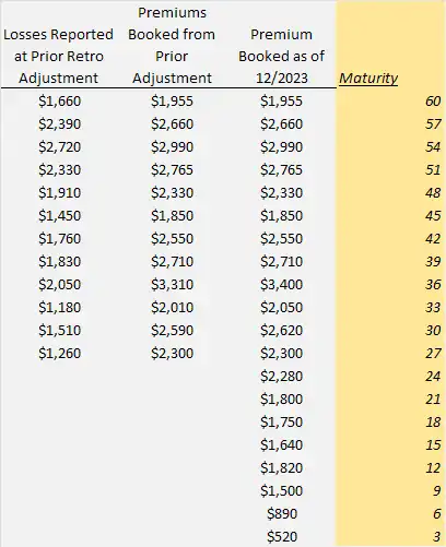
It would make sense if you are not given the full triangle to create a column for maturity of each Policy effective quarter.
Notice how at 27 months for premiums, first retro adjustment takes place
The next at 27 months

Calculate PDLD and #CPDLD Ratios
\(E(\text{Future Loss}) =\text{Ult Loss} -\text{Loss a/o most recent retro adj.}\)
- % earned factor for the latest year → to account for the fact that policies aren't fully earned by the end of the year
  - If not given, state "I assume that, % earned 100%"
- Most recent retro adj. = prior retro adjustment
\(E(\text{Future Prem}) =CPDLD \times\text{E(Future Losses)}\) ← Corresponding values
- Refer to the top to understand how to map them properly
Ultimate premium = \(E(\text{Future Prem})+\text{Prem booked a/o most recent retro adj.}\)
\(\text{Prem Asset} =\text{Ultimate Prem} -\text{Latest Val. Prem}\) ← which is the diagonal prem

Mind the difference between the booked premiums for the ultimate premium calculation
- (4) has a/o most recent retro adjustment
- (5) is what is yet to be adjusted → latest valuation date (diagonal)

Future Premium (step 3) can be calculated in another way¶

Use \(\downarrow\) formula to find \(P_{3}\), premium at third adjustment

\[ P_{n} = [BP + (CL_{n}\times LCF)] \times TM \]

Then find ultimate premium \(P_{ult}\)

\[ P_{ult} = [BP + (CL_{ult} \times LCF)]\times TM \]

And subtract the both: \(E(\text{Future Prem})= P_{ult}- P_{n}\)

Next¶

Why not use development method on premiums? Why use PDLD?
1. Ultimate incurred loss can be estimated more quickly than retro premiums can be obtained. We get a better estimate sooner.
2. LOGICALLY, retro premiums depend on incurred losses → thus look at the connection between them, instead of just premiums
PROs of PDLD
- Based on rating formula → explainable
- Emphasis on Premium sensitivity (in line with regulatory procedures)
- Adapts to changes in retro parameters (other methods get distorted)
CON of PDLD
- Ratios are difficult to come by (as params vary by year, state and plan)

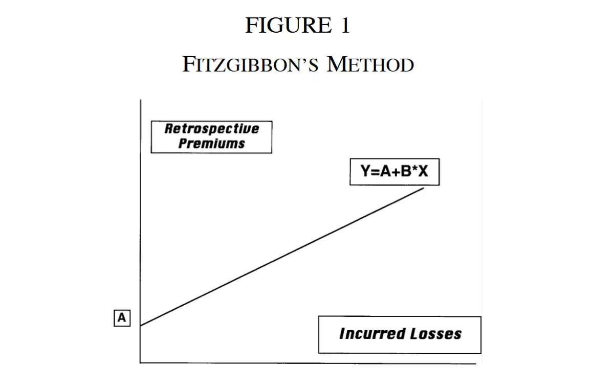
Fitzgibbon's method¶

To calculate premium asset, we use this reserve formula

\[ \text{Retro adjustment} = A + B \times \text{Standard Loss Ratio} \]

\(A\), \(B\) are estimated from historical regression
- \(A:\) intercept → minimum premium to cover expenses of writing and servicing policy
- \(B:\) slope represents the premium responsiveness
SLR and Retro adjustments from mature PYs (old)
\(\implies\) We don't need to calculate plan parameters in the PDLD method
CON:
- Doesn't consider emerging loss experience.
- Won't adjust the premium for worse or better loss experience at each premium adjustment.
- Problem 2: SLR doesn't account for the composition of losses (can be one very large loss or multiple smaller losses)

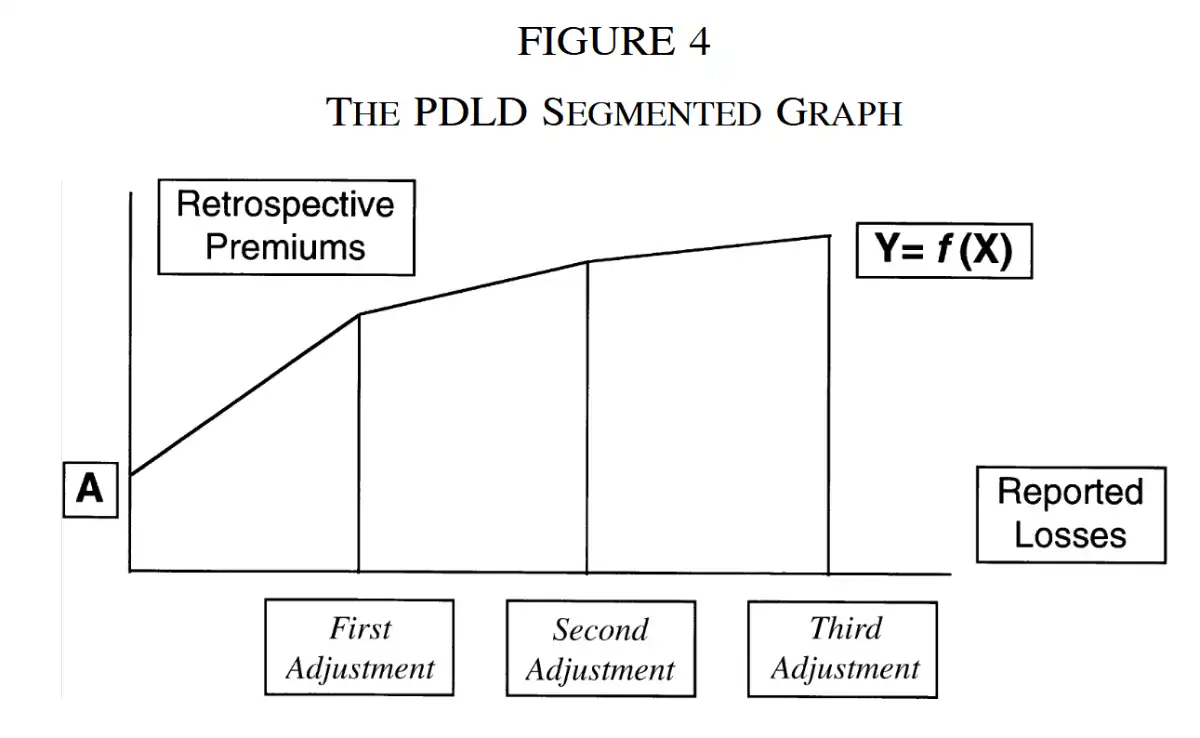
In contrast, for the PDLD method
- Premium responsiveness declines over time. Why? #later

Muffs¶

Be careful when calculating CPDLD ratio… you must divide by the total weights (when finding for \(CPDLD_{2+}\), the \% reported don't add up to 1)

Purpose: reduce risk from a loss ↩
If you write business thinking the claim frequency will be 100, but in the future during the policy period it turns out to be 150, its unprofitable ↩
Similar to PY but this is PQ (Policy Quarter) ↩