Stochastic Loss Reserving Using GLMs - Taylor

Study Strategy¶

Checklist¶

My Notes¶

Origin period: \(k\) reported in period \(j\)
\(Y_{kj}\) → Incremental \(j-1\) to \(j\)
\(X_{kj}\) → Cumulative losses
Experience period = calendar period
\(f_{kj}= \dfrac{X_{k,j+1}}{X_{kj}}\)
\(f_{j} = \sum_{k=1}^{K-j}w_{kj}f_{kj}\)

Exponential Dispersion Family¶

GLMs require a distribution from the EDF, which are of the form:

\[ \ln(\pi(y;\theta,\phi)) = \dfrac{y\theta-b(\theta)}{a(\phi)} + c(y,\phi) \]

\(y\) → Value of observation
\(\theta\) → Location/Canonical param
\(\phi\) → Dispersion/Scale param (like variance)
\(b(\theta)\) → Cumulant function → Shape
\(\exp(c(y,\phi))\) → normalizing factor, makes PDF integrate to \(1\)

Distribution	\(b(\theta)\) ← Link function	\(a(\phi)\)	\(c(y,\phi)\)	PDF
Normal (loss amt)	\(\dfrac{1}{2}\theta^{2}\)	\(\phi=\sigma^{2}\)	\(-\dfrac{1}{2}[\dfrac{y^{2}}{\phi}+\ln(2\pi \phi)]\)	\(\dfrac{1}{\sigma \sqrt{ 2\pi }}e^{ -1/2\left(\frac{y-\mu}{\sigma}\right)^{2} }\)
Poisson (claim counts)	\(\exp(\theta)\)	\(1\) (bcoz, variance = mean)	\(-\ln(y!)\)	\(\dfrac{\lambda^ke^{ -\lambda }}{k!}\)	KNOW THIS!
Binomial (loss amt/Freq)	\(\ln(1+\exp(\theta))\)	\(n^{-1}\)	\(\ln\binom{n}{ny}\)	\(\binom{n}{x}p^x(1-p)^{n-x}\) where	\(y = \dfrac{x}{n}\) and \(\theta = \ln(\dfrac{p}{1-p})\)
Gamma (loss amt)	\(-\ln(-\theta)\)	\(v^{-1}\)	\(v\ln(vy)-\ln(y)-\ln(\Gamma v)\)	\(\dfrac{1}{\Gamma(\alpha)\theta ^\alpha}x^{\alpha-1}e^{ -x/\theta }\)
Inverse Gaussian (loss amt)	\(-(-2\theta)^{1/2}\)	\(\phi\)	\(-\dfrac{1}{2}[\ln(2\pi \phi y^3+\dfrac{1}{\phi}y)]\)	\(\sqrt{ \dfrac{\lambda}{2\pi x^3}\exp(-\dfrac{\lambda(x-\mu)^{2}}{2\mu^{2}x}) }\)

Tweedie Sub-Family¶

EDF where \(V(\mu) = \mu^p\) where \(p \notin (0,1)\)
restrict \(a(\phi)=\phi\)
\(Var(Y)=\phi \mu^p\), variance is \(\propto\) a power of the mean

Distribution	\(p\)	\(b(\theta)\)	\(\mu\)
Normal	\(0\)	\(\dfrac{1}{2}\theta^{2}\)	\(\theta\)
Over-Dispersed Poisson	\(1\)	\(\exp(\theta)\)	\(\exp(\theta)\)
Gamma	\(2\)	\(-\ln(-\theta)\)	\(-\dfrac{1}{\theta}\)
Inverse Gaussian	\(3\)	\(-(-2\theta)^{1/2}\)	\(-(-2\theta)^{1/2}\)

ODP¶

\(E(Y)=\lambda\)
\(Var(Y)=\phi\lambda\)
Traditional Poisson has \(\phi=1\)
To be used when we don't have much idea about the distribution
Has the simplicity of traditional Poisson and flexibility due to \(\phi\)

Stochastic Models Supporting the Chain Ladder Method¶

Chain Ladder provides the MLE of loss reserves.

Non-parametric Mack Model¶

Prior Mack Assumptions with "For each AY, losses form a Markov chain" (Loss in one period only depends only on the losses in the period immediately prior and nothing else)
LDFs are MVUE (among Linear combinations of LDFs)

Parametric (EDF) Mack Models¶

We get the EDF Mack Model if we change the OG variance assumption to

\(C_{k+1}\) follows an EDF distribution

EDF Mack Model + Full triangle (\(\#AY = \#\text{Dev Periods}\)) ensures

MLEs of LDFs = Chain Ladder's LDFs
MLEs of LDFs are Unbiased

Additionally, if EDF is restricted to ODP (ODP Mack Model)

OG Chain Ladder LDFs are MVUE
\(\hat{C}_{j+1}\) and reserve estimates are also MVUEs

Cross-Classified Models¶

The incremental losses are independent
The incremental losses have a distribution belonging to EDF
\(E[Y_{kj}] = \alpha_{k}\beta_{j}\) where \(Y_{kj}\) is the incremental loss and \(\beta_{j}\gt 0\)
\(\sum_{j=1}^{J}\beta_{j} = 1\)
Remove redundancy with \(\beta_{1}=0\) or \(\alpha_{1}=0\)

Basically, we have both row and column parameters here.

If…

Full triangle
EDF is restricted to ODP
\(\phi\) is identical for all cells

Then…

MLE \(X_{j+1}\) and reserves = Chain Ladder estimates
If \(X_{j+1}\) and reserves are corrected for bias \(\implies\) MVUEs
Reserve estimates: ODP Mack = ODP Cross-Classified

Process¶

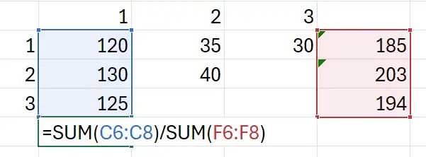
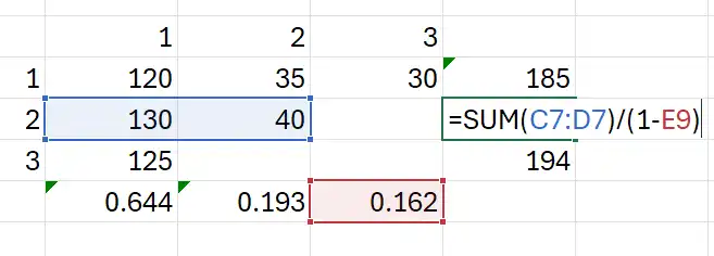
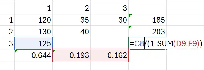
Also, we can calculate LDFs

\[ f_{j} = \dfrac{\sum_{k=1}^{j+1} \beta_{j}}{\sum_{k=1}^{j} } = \dfrac{0.644+0.193}{0.644} \]

Generalized Linear Models¶

Such¹ stochastic models can be represented as GLMs.
Useful information is returned by statistical software

\[ X = \begin{bmatrix} 1 & 0 & 0 & 0 & 0 \\ 0 & 1 & 0 & 0 & 0 \\ 0 & 0 & 1 & 0 & 0 \\ 1 & 0 & 0 & 1 & 0 \\ 0 & 1 & 0 & 1 & 0 \\ 1 & 0 & 0 & 1 & 1 \\ \end{bmatrix} \]

\[ A = \begin{bmatrix} \alpha_{1} \\ \alpha_{2} \\ \alpha_{3} \\ \beta_{2} \\ \beta_{3} \\ \end{bmatrix} \]

Thus,

\[ h(\mu) = XA \]

\(h(\cdot)\) → Link function
Traditional weighted LR model \(\downarrow\)

\[ Y_{i} = XA + \epsilon_{i} \text{ with } \epsilon_{i} \sim N(0, \phi_{i}) \]

GLM is a generalized version where
- Relation between \(X\) and \(Y\) may be non-linear
- Error terms may be non-normal
Params of \(A\) are estimated using MLE
\(\phi\) is unknown and usually assumed to be \(\phi_{i} = \dfrac{\phi}{w_{i}}\)
- \(w_{i}\) is a known weight given to each observation
- Required to calculate \(Var(Y) = a(\phi)V(\mu)\)
GLM requires
- \(b(\theta)\) → model's assumed error distribution
- \(p\) → mean-variance relation
- Covariates → influencing \(\mu\)
- \(h(\cdot)\) → functional relationship b/w \(\mu\) and covariates

Covariates¶

Categorical covariates used in \(X\) (specify which accident year and development year)
- \(\alpha\) → AY
- \(\beta\) → Dev periods
Continuous variate
- age instead of AY
- linear spline \(L_{mM}(x) = min[M-m, max(0,x-m)]\)

GLM Representations of the Chain Ladder Method¶

Solve using Chain Ladder

If given characteristics of a GLM model that fit requirements to match the chain ladder output → SOLVE using Chain Ladder, don't setup a GLM.

Parametric Mack Model¶

\[ Y_{k,j+1}|X_{kj} \sim ODP(\mu_{kj},\phi_{j}) = ODP((f_{j}-1)X_{kj},\phi_{j}) \]

Note that \(\phi_{j}\) doesn't vary by AY

ODP Cross-Classified Model¶

\[ Y_{k,j+1}|X_{kj} \sim ODP(\mu_{kj},\phi_{j}) = ODP(\alpha_{k}\beta_{j},\phi) \]

Note that \(\phi\) doesn't vary at all

Deviance¶

\(D(Y,\hat{Y}) = 2 \sum_{i=1}^{n}[\ln[\pi(Y_{i}, \hat{\theta}^{(s)},\phi)]- \ln[\pi(Y_{i};\hat{\theta},\phi)]]\)

Residuals¶

\[ R_{i}^{p} = \dfrac{Y_{i}-\hat{Y}_{i}}{\hat{\sigma}_{i}} \]

Adjustments to the Model¶

Heteroscedasticity¶

Plot of residuals, aren't evenly spaced
Use non-constant values for \(\phi\)
Taylor mentions weighting the scale parameter differently

Outliers¶

Use weights (0 → Outlier)
Ensure we are not removing events that reflect potential future variability

Using only Recent Experience¶

Set weights for observations outside the last \(n\) diagonals to \(0\).

For which chain ladder results are MLE ↩