Using the ODP Bootstrap Model - Shapland

Study Strategy¶

Get the simple idea about bootstrapping first and apply it on a triangle. Put it in excel. That way you will see the connect about the \(H\) hat matrix and stuff
Understand that once we have built a foundation about the bootstrapping process (as the first item in the checklist says), we will be able to learn the other concepts easily as those concept refer back to this process. So ensure that you spend some time understanding the bootstrapping process
Then you have to go through each of the "common modelling problems". To be honest, its quite straightforward, just have a read and focus on
- Why is it a problem?
- What is a solution to this problem?
Evaluation of models for reasonability → look and interpret graphs
Finally, the weighting and correlation section is much much much easier than it might initially seem. You just have to read through it once and follow through the examples (especially weighting section) then everything becomes clear
Finally, go through the various assumptions of the ODP model (they get referred to a lot, and it is useful to gather all that information in one place and get an overall idea how in different contexts (modelling problems etc) these assumptions play a role)
Also try to see the connection between chain ladder and ODP model (and reason out why ODP is preferred even if they give the same output)

Checklist¶

My Notes¶

Notation¶

\(c(w,d)\) → cumulative losses
\(q(w,d)\) → incremental loss from \(d-1\) to \(d\)
\(m(w,d)\) → expected incremental losses from \(d-1\) to \(d\)
\(r_{w,d}\) → residual

GLM Bootstrap Process¶

https://docs.google.com/spreadsheets/d/1cbQT4SFuCTMMxs5i1zSnWjxBPNv1CAyYSFELD6_GIhw/edit?usp=sharing

Multiple samples through resampling

Steps¶

\(\text{Triangle}\)
\(\log(\text{Triangle})\) ← Log link triangle
System of equations

	1	2	3
1	\(\alpha_{1}\)	\(\alpha_{1}+\beta_{2}\)	\(\alpha_{1}+\beta_{2}+\beta_{3}\)
2	\(\alpha_{2}\)	\(\alpha_{2}+\beta_{2}\)
3	\(\alpha_{3}\)
- Least squares and MLE to solve for \(\alpha_{w}\) and \(\beta_{d}\) params

Residuals¶

The big idea

We compute the unscaled Pearson residuals, and compute an adjustment factor \(f^H_{w,d}\) ← \(H\) ← \(W\) and \(X\), to convert them to standardized Pearson Residuals.

Unscaled + Adjustment → Standardized

Unscaled Pearson residuals, \(r_{w,d}\):

\[ r_{w,d} = \dfrac{q(w,d) - m_{w,d}}{\sqrt{ m^z_{m,d} }} \]

\(z\)	Dist
0	Normal
1	Poisson (ODP)
2	Gamma
3	Inverse Gaussian

Hat matrix \(H\):

\[ H = X(X^T WX)^{-1}X^TW \]

where,

\[ W = \begin{bmatrix} m_{1,1} & 0 & 0 & 0 & 0 & 0 \\ 0 & m_{2,1} & 0 & 0 & 0 & 0 \\ 0 & 0 & m_{3,1} & 0 & 0 & 0 \\ 0 & 0 & 0 & m_{1,2} & 0 & 0 \\ 0 & 0 & 0 & 0 & m_{2,2} & 0 \\ 0 & 0 & 0 & 0 & 0 & m_{1,3} \end{bmatrix} \]

In excel,

=mmult(X,inverse(mmult(transpose(X),W,X)),transpose(X),W)

Adjustment factor

\[ f_{w,d}^H = \sqrt{ \dfrac{1}{1-H_{i,i}} } \]

Standardized Pearson residual: \(r^H_{w,d} = r_{w,d} \times f^H_{w,d}\)

Sampling¶

We have a set of standardized residuals, from which we can sample.

We ignore any zero-value residuals, because they arise due to the parameter that applies only to that particular cell. Thus (expected = actual). But we assume that those cells will actually have some variance which is unobserved now. Thus we sample from other non-zero values.

And form the triangle, next calculate sampled incremental values

\[ q^*(w,d) = r^* \times \sqrt{ m^z_{w,d} } + m_{w,d} \]

Then calculate LDFs
→ Ultimate losses and Estimated Reserves

Process Variance (\(z=2\), Gamma)¶

Using Gamma Distribution, we will do probabilistic sampling

\[ E(x) = m_{w,d} \quad Var(x) = \phi m^z_{w,d} \]

where \(\phi\) is the scale parameter:

\[ \phi = \dfrac{\sum r^2_{w,d}}{N-p} \]

\(N\) → number of cells in triangle
\(p\) → # of \(\alpha\)'s and \(\beta\)'s

\[ \phi = \dfrac{\sum(r^H_{w,d})^{2}}{N} \]

Select probability \((0,1)\) for each incremental cell to be sampled
Compute \(\beta = \phi\) and \(\alpha =\dfrac{m_{w,d}}{\phi}\)
gamma.inv(probability, alpha, beta)

ODP Bootstrap \((z=1)\)¶

We don't need to solve for the \(\alpha_{w}\) and \(\beta_{d}\) params in the beginning.
\(E(\text{Ult})\) ← Latest diagonal & divide by volume-weighted LDFs
We can arrive at the same expected values using LDFs (since \(z=1\) and its a Poisson distribution) (we also need \(\beta_{1} = 0\) and no additional params)

GLM Bootstrap¶

No requirement regarding number of parameters
- Simplify by combining accident (development) years to have fewer accident (development) year parameters
- Can add calendar year parameters to explain calendar year effects
- Solve for parameters using least squares or MLE \(\alpha_{w}\) and \(\beta_{b}\) → \(m_{w,d}\) and the same process follows
Advantages (GLM with diff params)
- Avoid over-fitting, flexibility to capture trends
- Fewer params allow corner residuals to be variant (non-zero) and allow for sampling
- Calendar year trends can be added
- Can work even if its not a complete triangle
Disadvantages (GLM with diff params)
- After each iteration, re-solving for \(\alpha_{w}\) and \(\beta_{d}\) is required
- LDF explicability is lost

Common Modelling Problems¶

1. Negative incremental values¶

Prefer paid over incurred → negative incremental values are less likely
Adjust triangle
1. Sum of each column of incremental numbers should sum to zero
  - Adjust log-link function: take \(\ln(\text{absolute value})\) or \(0\)
2. If not
  - Add such a number (say 30000) to every cell that will lead to all values being \(\geq 0\) (if the largest negative number is -30000)
3. From the fitted incremental values, subtract the number (30000) ← Reverse adjustment
Unscaled residual formula

\[ r_{w,d} = \dfrac{q(w,d) - m_{w,d}}{\sqrt{ abs(m^z_{m,d}) }} \]

Sampled incremental formula

\[ q^*_{w,d} = r^* \times \sqrt{abs(m^z_{m,d})} + m_{w,d} \]

2. Non-zero mean of residuals¶

Since residuals are random observations of the true residual distribution, they don't always average to zero (which they should in the model)
Case 1: Significantly different from zero → Model probably ain't a good fit
Case 2: Close to zero: Should we adjust?
- Yes or For adjusting → residuals with positive (negative) average will increase variability and increase (decrease) the total resampled losses.
- No or Against adjusting → non-zero average is a characteristic of the data and shouldn't be meddled with

To adjust, add a constant to each cell

\[ a_{w,d} + c \to \text{such that average = 0 } \forall w,d \]

3. Using an L-year weighted average¶

We want to use last 3/5/L years
Selectively sample residuals for the last L+1 diagonals rather than the entire triangle.
- Set rest of the residuals to 0
For ODP Bootstrap, we need to sample the entire triangle to → sum everything together and get cumulative losses to calculate LDFs (YOU NEED THE ENTIRE TRIANGLE BRO)

4. Missing values¶

A more general GLM is less impacted
For ODP, its bad. LDFs become challenging to calculate
If latest diagonal values are missing \(\implies\) We won't be able get the fitted triangle at all.
Solutions
1. Impute
2. Modify LDF to exclude missing values
3. If most recent diagonal value(s) missing → estimate the value or use 2nd most recent diagonal to calculate fitted values

5. Outliers¶

Outliers don't represent the variability we expect to see in our data in our future.
Options
- Remove and treat them as missing
- Exclude from LDFs, but still randomly sample residuals for that cell \(\implies\) use the sampled non-extreme values.

Be sure!

Ensure that the outlier actually doesn't represent expected variability in future data.

6. Heteroscedasticity¶

GLM Bootstrap assumes that residuals are IID (This allows us to sample a residual from \(w,d\) and use it for \(w',d' \neq w,d\))
But IRL, some dev periods may have residuals with more variance than others (violation!)
We need to account for the credibility of observed differences. #doubt
- Compare variance in residuals: dev period with 2 vs 10 residuals
Heteroskedasticity \(\implies\) not a good fit. Adjust GLM bootstrap parameters to improve fit.

But for ODP Bootstrap models,

For ODP we don't have this flexibility.
Downside of ODP → overparameterization
Standard deviations \(\sigma\) differ by development period significantly
- \(\implies\) Group development periods: 1-3, 4-7 and 8-10 (for credibility)

ODP Bootstrap adjustments for heteroskedasticity¶

Stratified sampling
- Group dev periods with homogenous variances
- Sample only from the residuals in each group (if we are sampling for cols 1-3, then choose residuals in columns 1-3)
- Pro
  - Straightforward
- Cons
  - Some groups have few residuals in them… limits amount of variability.
  - Partially defeats the purpose of random sampling with replacement
Calculating hetero-adjustment parameters
- Adjust residuals so that they become homoscedastic, then undo the adjustment from sampled incremental values
- Hetero-adjustment, \(h_{i} =\dfrac{\text{standard deviation for the whole triangle}}{\text{standard deviation for the group}}=\dfrac{\text{total}}{\text{individual}}\)
- \(r^*_{w,d} = r_{w,d} \times f_{w,d}^H \times h_{i}\) (assuming \(z=1\))
- "Unadjust" residual back to the variance for column 3
  - \(q^{i*}(w,d) = \dfrac{r^*}{h_{i}}\times \sqrt{ m_{w,d} } + m_{w,d}\)
- Pro
  - Sample from entire pool of residuals
- Cons
  - Hetero-adjustment parameters → overparameterized
Calculating non-constant scale parameters \(\phi\)
- Calculate scale parameter for the whole triangle: \(\phi = \dfrac{\sum r^{2}_{w,d}}{N-p}\)
  - \(\phi = \dfrac{\sum\left( \sqrt{ \frac{N}{N-p} }\times r_{w,d} \right)^{2}}{N}\) (equivalently)
- \(\phi_{i} = \dfrac{\frac{N}{N-p}\times \sum_{i=1}^{n_{i}}r^{2}_{w,d}}{n_{i}}\), \(n_{i}\) → residuals in a group
- Adjustment factor: \(h_{i} = \dfrac{\sqrt{ \phi }}{\sqrt{ \phi_{i} }}\)
- See an “Example” (pdf) for calculation

7. Heteroecthesious data¶

"Heteroecthesious" → different exposure periods
Due to
1. Partial first dev period (first column covers shorter time span)
  - Requires very little adjustment
  - Use Pearson residuals
2. Partial last calendar period (last diagonal) #doubt
  - For latest AY, multiply the projected future payments by the portion of exposures in first dev period (1/2)
  - Reduces the projects to remove future exposures

8. Increasing or Decreasing exposures¶

If exposures have changed significantly over the years.
Divide claim data by earned exposures of accident year (at the beginning before any other steps are taken)
This adjustment helps us use fewer accident year parameters in the model.

9. Tail factors¶

If claims do not reach full development, we need tail factors
Can also set a distribution around a tail factor.

10. Lack of residuals¶

If there are limited number of residuals, we won't know if there is enough variability in our model.
Solution: Parametric bootstrapping → Fit a distribution to the residuals and sample from entire distribution.

Diagnostics¶

Evaluate for fit. Nothing called "perfect", but we want a reasonable representation of our data.
Not to find the "best" but to find a set of reasonable models that can be weighted together as discussed in #Weighting Methods Together.

Residual Graphs¶

Plot residuals against
- Acc Period
- Dev Period
- Payment period
- Predicted Losses
Residuals random around zero.
- If not roughly 0 \(\implies\) \(\exists\) un-modeled trends
- If variance is not similar around zero \(\implies\) Heteroscedasticity

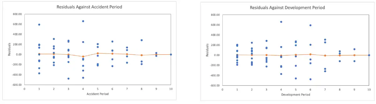
These graphs are from data showing heteroscedasticity \(\uparrow\)

Normality Test¶

Compare residuals to a normal distribution (to check skewness)
If normality looks better before the heteroscedasticity adjustment \(\implies\) The fit of the model wasn't really improved.¹

Outliers¶

Significant number of outliers \(\implies\) model isn't a good fit.
Use the box-whisker plot to check for outliers
- Box = middle 50th percentile of the residuals (25th to 75th)
- Whiskers show 3 times the IQR
- Residuals beyond the whiskers → outliers
Decide whether you want to remove outliers or not
Or see if any other adjustments provide a better fit with fewer outliers

Reviewing Model Results¶

The point

Evaluate trends in standard error and CV

After other diagnostic tests, select acceptable models & run simulations for each of them

AY	Mean Unpaid	Standard Error	CV
2007	94649	96571	102.0%

Patterns to look for when looking at \(\uparrow\) table:

SE should increase from oldest to most recent years ← Magnitude of error should increase with mean
Total SE \(\gt\) any Individual SE
CV should decrease from oldest to most recent
- Because of independence in claim-payment stream (note this point)
- There will be many claim payments for a recent CY, and thus variability of one will get offset by another. Thus, the variance of the overall would be less, because the total would be more or less as per expectation.
- Possible if CV comes up in the most recent years. Because
  1. More parameters at play in most recent years \(\implies\) parameter uncertainty \(\gg\) process uncertainty
  2. If increase is significant → Uncertainty might be overestimated → may benefit from another model.
Total CV \(\lt\) any individual year
Last point #doubt

Weighting Methods Together¶

A practical way of addressing model risk by NOT being overly dependent on any single model

Alternate Methods¶

Problem with ODP

Most recent AY → Highly volatile results (like LDF method, a high/low initial observation leverages the projected ultimate)

Use bootstrapping to correct for this by
Finding a distribution around the dev factors.
Use Bornhuetter Ferguson or Cape Cod technique

Given the distribution of Ultimate Expected Losses

Cumulative Dist	Ultimate Expected Losses
50%	50000
100%	60000

Determine expected losses.
- If random number \(\leq\) 0.5 → Use 50000
Determine the percent unreported.
- If given in problem, use that
- Else compute from distribution given (like that of cumulative distribution in this case)
- Or compute from LDF = \(1 - \dfrac{1}{\text{Cum LDF}}\)
Calculate Reserves using BF method
- \(\text{ultimate} \times\text{\% unreported}\)

Combining Methods¶

Given a choice of models, how do we combine them? Shapland suggests:

Run models with same random variables, and take weighted average of all outputs
- e.g. ODP bootstrap method is run using Chain Ladder and B-F GLM Bootstrap is also run
  - All models used the same random variables
  - Estimates (unpaid loss) from each method is given
  - Weights from each method is given
  - Weighted average unpaid losses is also given
Run models with independent random variables, given each model a weight and then randomly select a model for each iteration
- e.g. Same situation as (1) but
  - Random variables are simulated independently of other models
  - Run two simulations
    1. Random number = 0.57 selected
    2. Random number = 0.29 selected
  - Estimates (unpaid loss) for each model is given (for each simulation #1 and #2)
  - Weights for each models are given
- Solution → according to the weights, use the random number to decide which number model to select for each simulation
  - Simulation #1 → select BF
  - Simulation #2 → select CL
  - Then take a straight average of BF numbers from (Sim #1) and CL numbers from (Sim #2)

Correlation¶

We need a single estimate for the entire business (aggregating various LOBs) but the challenge is that there is correlation between LOBs.

Location Mapping¶

Takes place during residual sampling, for first LOB, make a note of the location of the sample… and sample the other LOBs from the same location (e.g. AY 2023, Dev Period 1 → Row 5, col 3. Then for another LOB AY2023, Dev period 1 also should come from Row 5, col 3). This keeps the correlation constant.

Pros
- Simple to implement
- No need to estimate correlation matrix
Cons
- Requires business segments to share same data triangle shape (no missing values/outliers)
- Can't use other correlation assumptions to stress test the model #doubt

Re-sorting¶

Calculate the correlation matrix. Resort the residuals based on correlations. Recommended to use Spearman's Rank Order, Iman-Conover or Copulas for correlation and resorting process

Pros
- Allows different shaped triangles
- Different correlation assumptions can be tested
- Using different correlation algorithms → other benefits on aggregate distribution.

Sometimes just by changing the hetero groupings improves the fit of the model (by hit and trial, which can be taken up using this normality test). ↩