Stochastic Loss Reserving Using Bayesian MCMC Models - Meyers

Study Strategy¶

Just get a hang of interpreting the \(p\)-\(p\) curves properly. Understand what light and heavy tailed means using examples (read the footnote and the illustration provided. But have your own way to explain it)
Understand what Bayesian MCMC is all about → Just a neat way to find parameters
Read each of the model with the overview in the next bullet.
There are 5 models. Some are fit to incurred data, and perform decently well. But with paid data only CSR performs well (\(\implies\) paid data doesn't have that information and that is what creates the bias.)
- Leveled or correlated
- with Trend (leveled or correlated)
- with CSR

Checklist¶

My Notes¶

Pronounced as "Mayas"

CL is MVUE but does it have the best predictive power? Or can something be improved?
Mack and ODP model failed to model. Why a model may not perform well?
- Insurance environment is too dynamic for one model fits all.
- There can be other models that fit the data better
- Data might be missing information
  - e.g. changes to business practices, claims processes or reinsurance treaties

Meyers' Process¶

He pulled losses from Schedule P of the NAIC Annual Statements of 50 different companies for each line of business (200 companies) → CA, PA, WC, OL → incurred/paid/both depending on model
Use Loss dev triangles (last year = 1997). He runs as if today is Jan 1998, to compare predicted future losses to actual.

Interpreting percentiles

Meyers finds the mean and standard deviation of incurred losses using his model
Then he looks at the actual loss amount and asks "What is the percentile of this observation in the distribution I just calculate above?"

Validation Models¶

A histogram groups data into evenly-sized "buckets" and then graphs the frequency of outcomes in each.
- Look for bars approximately equal in height
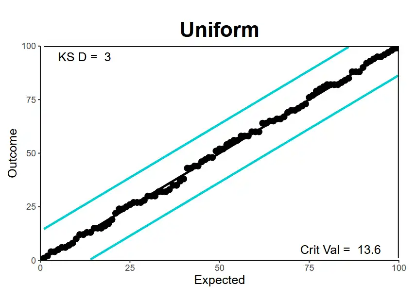
\(p\)-\(p\) plots and Kolmogorov-Smirnov test → Differences between where the point is and where we expect it to be. (\(n\) → Number of data-points)
- \(\{ p_{i} \}\) set of actual percentiles → Ascending order
- \(\{ f_{i} \}\) set of expected percentiles \(= 100 \times \{ \frac{1}{n}, \frac{2}{n},\dots \frac{n}{n} \}\)
- \(\dfrac{136}{\sqrt{ n }}\) → critical value at 5% significance
- Find the maximum absolute difference \(D\) → \(\max\lvert p_{i} - f_{i} \rvert\) which has to be compared to critical value. If the \(D\) is smaller → Model passes the test!
- Include lines on the \(p\)-\(p\) plot to show critical value boundaries
Anderson-Darling Test
- More sensitive to the fit of extreme values
- Doesn't discuss much because all his models fail the test → Can be used in the future if someone comes up with a more refined model

Graph	Description	Verbal Summary
Uniform	Not perfectly flat but enough, randomly fluctuating at the tops.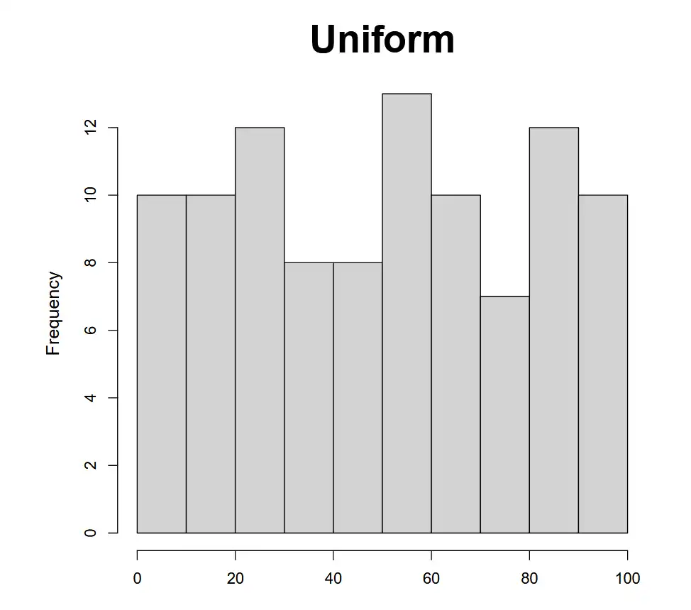
Light tailed	Predicts² too few values in the tails. When modeled standard deviation is too low.¹	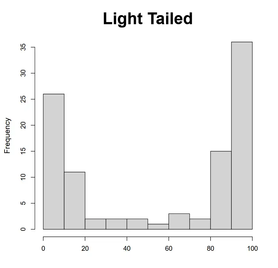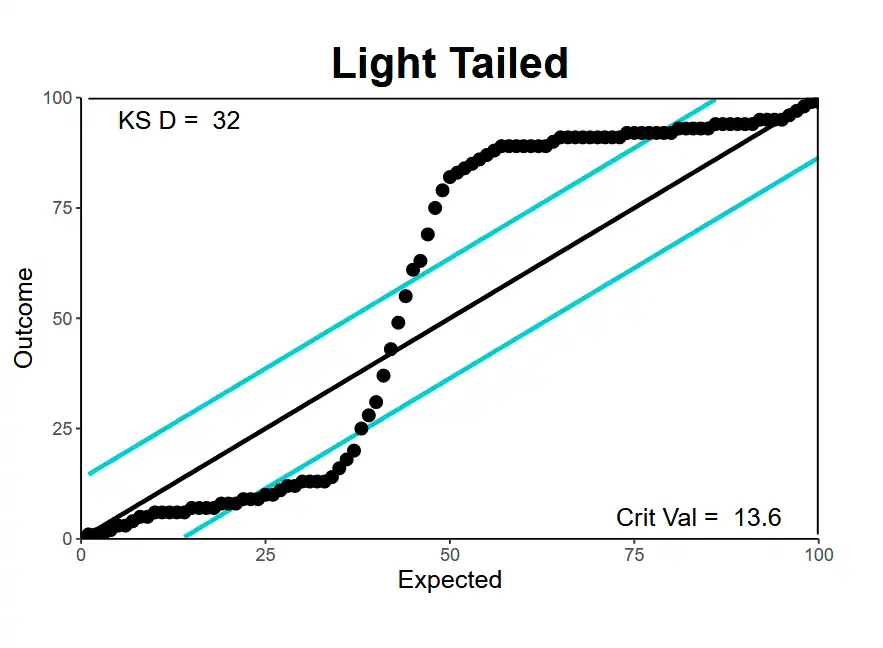Left side: actual values are smaller (3,5,7) than expected ones (5,6,7). And vice-versa on the right.
Heavy tailed	Predicts too many values in the tails (too few in the middle) → Standard deviation is too high³	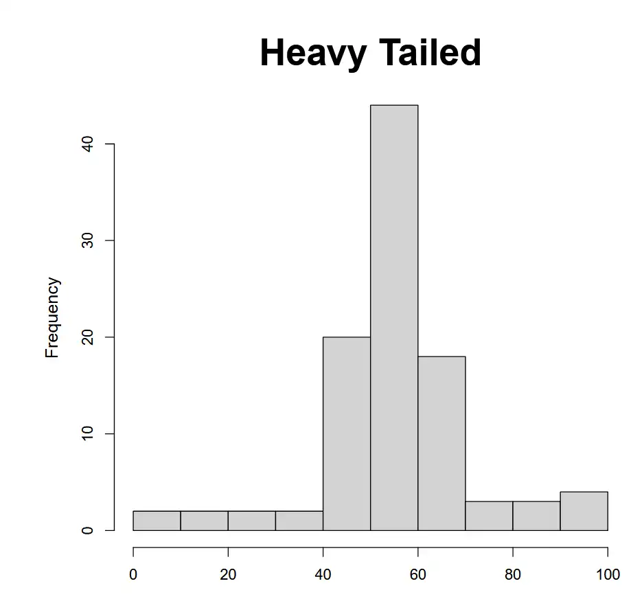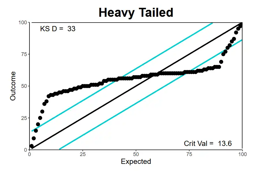Reverse of \(\uparrow\). Should have less number of observations in the tails
Biased High	Estimate majority of losses higher than they actually are. Mean is too high.	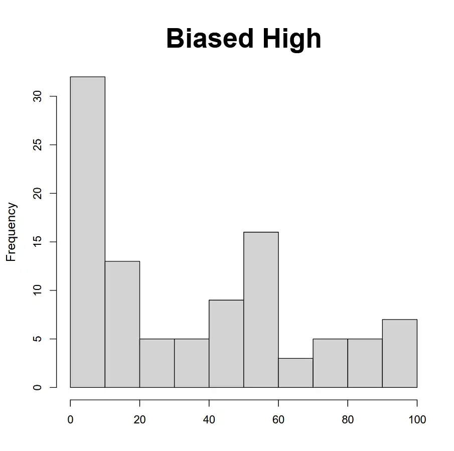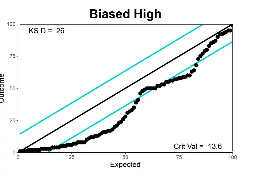All observations are overestimated! (Biased high!)

An illustration to the concept of standard deviation \(\downarrow\). This is light tailed because we needed more in the tails (e.g. 3,5) to match reality than we expect (5,6).

We can also have a biased low model but Meyer's doesn't find any.

Existing Models¶

Mack Model with Incurred data
- PA, CA, OL → Pass
- WC → Fails
ODP Bootstrap with Paid data
- Using paid ← Bootstrap model uses log of incremental losses and incurred is more likely to have negative (as case reserves are adjusted) and we cannot have log of negative incremental loss
- \(E(q_{w,d}) = \alpha_{w}\beta_{d}\) and \(Var(q_{w,d}) = \phi \alpha_{w}\beta_{d}\)
- CA, OL → Pass
- PA, WC → Fail

Width of the band

Critical value of all lines is smaller than the individual LOBs because \(n=50\) for individual lines and \(n=200\) for all lines combined. And critical value = \(\dfrac{136}{\sqrt{ n }}\)

Bayesian MCMC¶

These models rely on Markov chains → random processes where the transition to the next state depends only on its current state. (e.g. Metropolis Hastings algorithm)
Basic steps
1. Select → Prior & Conditional distribution
2. Select → starting vector. Run large number of iterations, with various phases:
  - Adaptive phase → improve model efficiency
  - Burn-in phase → help model start to converge
  - Final phase → for sampling
3. Take sample from final phase and update posterior distribution from this sample.

LCL Model (Incurred)¶

Leveled means AYs are uncorrelated!

Similar to ODP Bootstrap model but Bayesian MCMC method to solve for parameters.
- \(\mu_{w,d} = \alpha_{w} + \beta_{d}\)
- Cum losses → Lognormal distribution (log mean \(\mu_{w,d}\) and log SD = \(\sigma_{d}\))⁴
  \(\sigma_{1} \gt \sigma_{2} \gt \dots \gt \sigma_{10}\)
- \(\beta_{10} = 0\) for unique solution
- Assign remaining \(\beta_{d}\) to a wide prior distribution⁵

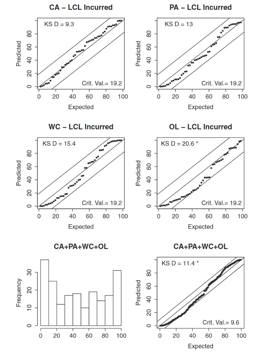
Observation

Light tailed but not as much as the Mack model

CCL Model (Incurred)¶

Base is #LCL Model (Incurred) and adds a between-year correlation
- \(\mu_{1,d} = \alpha_{1} + \beta_{d}\)
- \(\mu_{w,d} = \alpha_{w} + \beta_{d} + \rho(\ln(C_{w-1,d})- \mu_{w-1,d})\) for \(w\gt 1\)
  - \(\alpha + \beta + \rho(\ln\text{actual}- \ln\text{expected})\) from the previous AY
- Rest is the same as LCL so if \(\rho=0\) \(\implies\) Same as LCL model
E.g.
- Compute \(\mu_{2019,60}\) and use it to compute \(\mu_{2020,60}\) using params \(\alpha_{2020}\), \(\beta_{60}\) and \(\rho\) along with the actual value of \(C_{2019,60}\) and the expected value we just calculated \(\mu_{2019,60}\).

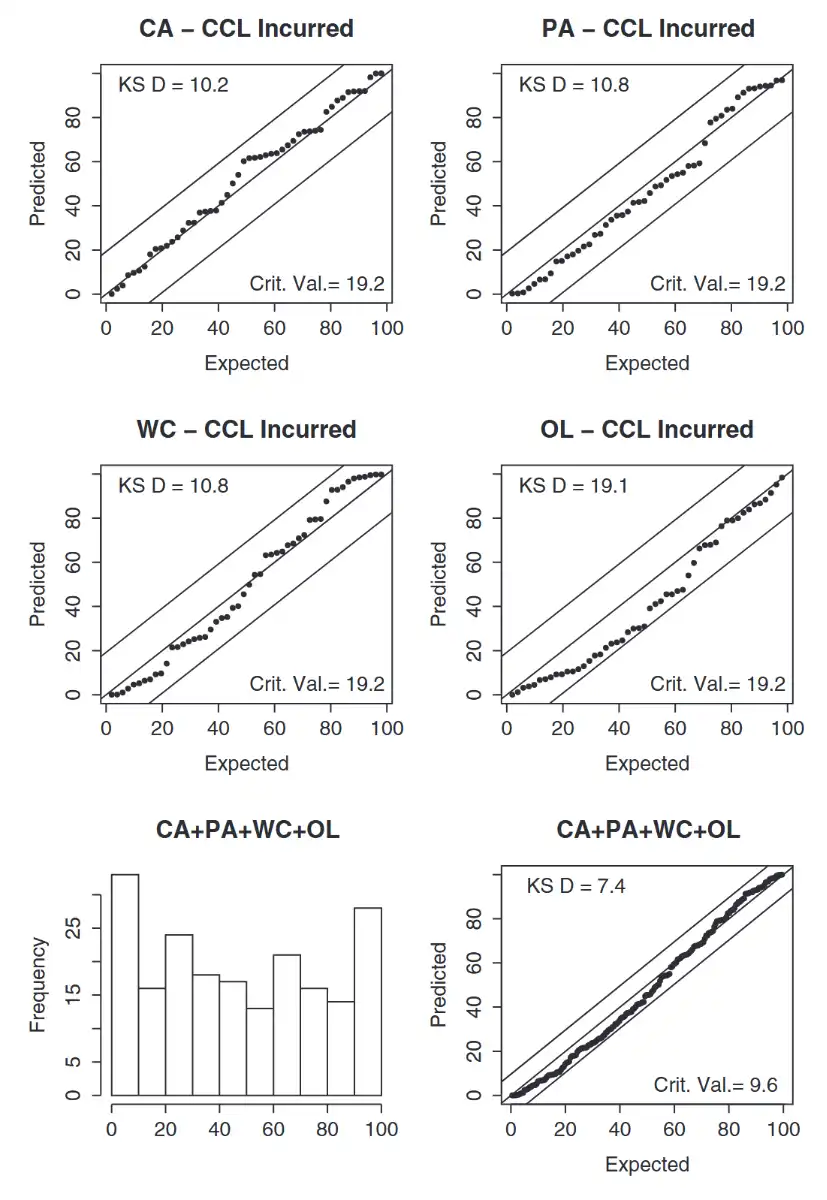
Observation

Passes K-S test individually and in total (just barely in OL)
Larger standard deviation than Mack model
Lean lightly to the light-tailed side

CCL Model (Paid)¶

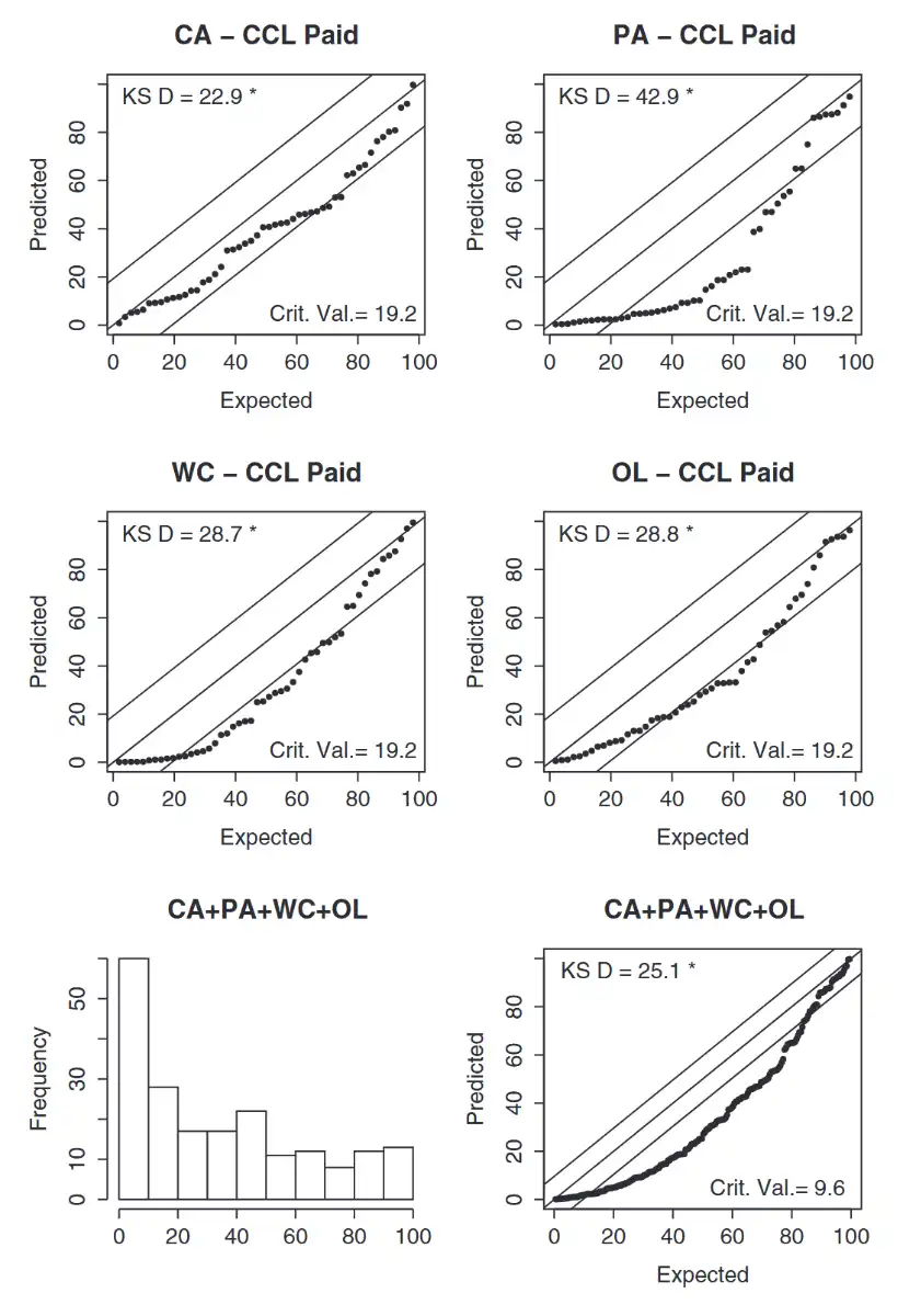
Observation

Terrible and biased high!

CIT Model (Paid)¶

Includes a payment year trend
Based on incremental paid (not cumulative paid) → since cumulative will include already settled claims (that won't change) and we just want to look at the part of claims data that changes.
Incremental paid tends to be skewed right and negative (sometimes). Two distributions that allow for that
1. Skew Normal distribution
  - \(\mu\) → location param
  - \(\omega \gt 0\) → scale parameter
  - \(\delta\) → shape parameter, \(\in (-1,1)\)
  - Combination of truncated normal distribution and normal distribution (\(\delta = 0\) \(\implies\) Normal)
  - Con: We need a more skewed distribution (since \(\delta\) is close to 1 for most incremental triangles and \(\delta\) in the model is capped to \(1\))
2. Mixed log-Normal Normal
  - Also uses \(\mu\), \(\omega\), and \(\delta\)
  - Without limits to skewness → Allows for more accurate reflection of incremental paid loss triangles' skewness
CIT Model Characteristics
- \(\mu_{w,d} = \alpha_{w} + \beta_{d} + \tau(\omega - d - 1)\)
  - \(\tau\) (PAYMENT YEAR TREND TERM)
- Modelled incremental loss \(\tilde{I}_{w,d}\)
  - \(\tilde{I}_{1,d} \sim\text{normal}(Z_{1,d},\delta)\)
  - \(\tilde{I}_{w,d} \sim\text{normal}(Z_{w,d} + \rho(\tilde{I}_{w-1,d}- Z_{w-1,d})e^\tau,\delta)\) for \(w \gt 1\)
    - \(\rho\) (CORRELATION TERM)
- \(Z_{w,d} \sim\text{lognormal}(\mu_{w,d},\sigma_{d})\) where \(\sigma_{1} \lt \sigma_{2} \lt \dots \lt \sigma_{10}\)
  - Note that magnitude order of \(\sigma_{d}\) is reversed → Expect smaller, less volatile claims are settled earlier \(\implies\) more volatile claims paid later so \(\sigma_{1} \lt \sigma_{2} \lt \dots \lt \sigma_{10}\)
  - Compare it with before. For cumulative distribution → Volatility decreases over time since greater proportion of claims are settled \(\sigma_{1} \gt \sigma_{2} \gt \dots \gt \sigma_{10}\)
- Assign \(\beta_{d}, \alpha_{w}, \sigma_{d}\) and \(\rho\) to relatively wide prior distribution.⁵

Mixed lognormal normal distribution = lognormal \(Z\) distribution inside a normal distribution.

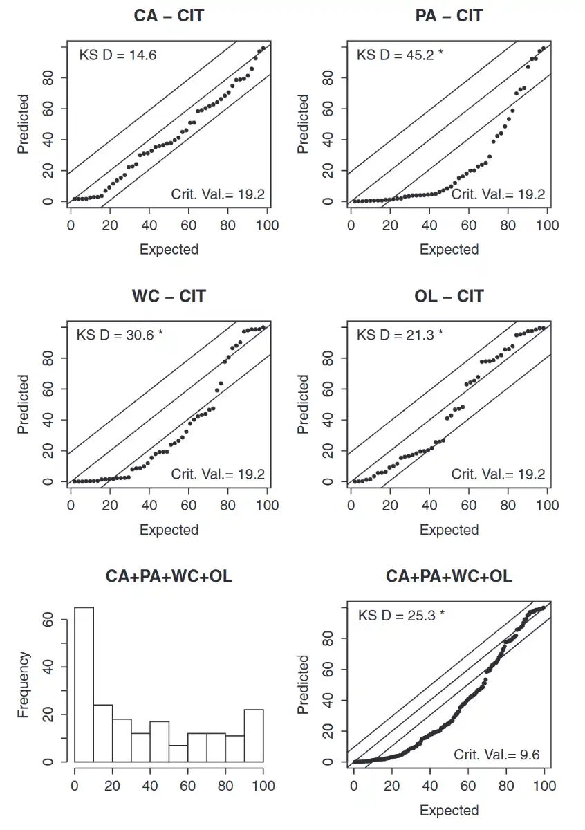
Observation

Model is biased high!

LIT Model (Paid)¶

Leveled means AYs are uncorrelated!

Identical to #CIT Model (Paid) but \(\rho=0\)

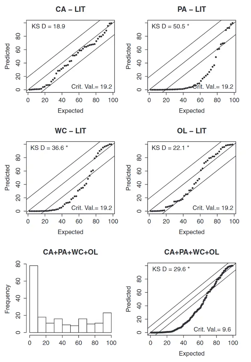
Observation

Model is biased high!

CSR Model (Paid)¶

Perhaps the paid data is missing information about speedup in claim settlement rates

Model
- \(\mu_{w,d} = \alpha_{w} + \beta_{d}(1-\gamma)^{(w-1)}\) where \(\gamma \sim\text{normal}(0,0.025)\)
- Model cumulative losses, \(C_{w,d} \sim\text{lognormal}(\mu, \sigma)\)⁴
- \(\beta_{10} = 0\) → for unique solution
- \(\beta_{d}\) to wide prior distribution⁵
Cumulative paid \(\uparrow\) so \(\beta_{d} \propto d\) and since \(\beta_{10} = 0\) \(\implies\) all our previous \(\beta\)'s are negative. Thus, \(\gamma \gt 0\) will ensure that \(\beta_{d}(1-\gamma)^{(w-1)}\) increases as \(w\) increases, indicating a speedup in claim settlements and vise-versa.
- \(\gamma \gt 0\) → speedup in CSR
  - \(\beta_{d}(1-\gamma)^{w-1}\) will start decreasing down \(w\)
  - -0.500
  - -0.495
  - -0.490
  - -0.485
- \(\gamma \lt 0\) → slowdown in CSR
  - \(\beta_{d}(1-\gamma)^{w-1}\) will start increasing down \(w\)
  - -0.500
  - -0.505
  - -0.510
  - -0.515

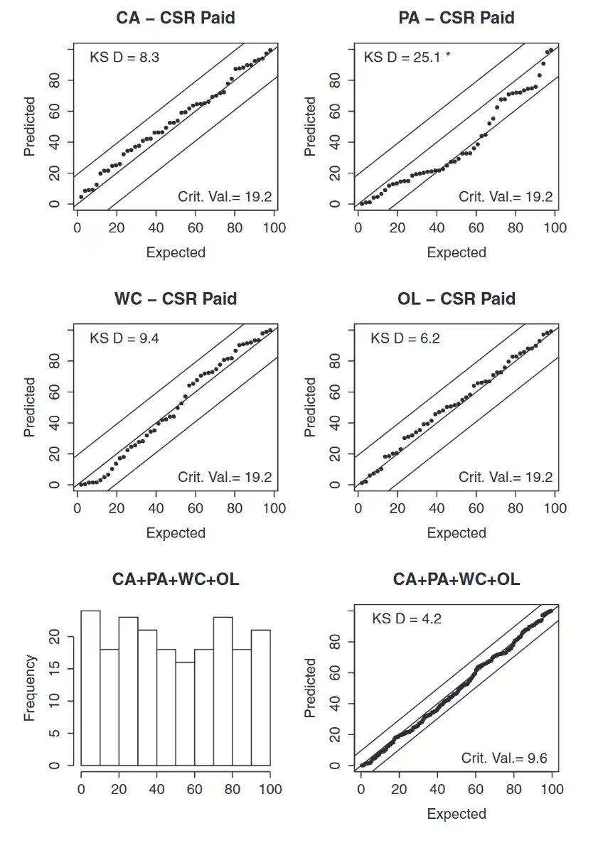
Observation

PA is still biased high
Corrects for the bias of other paid models → Incurred data recognized speedup of CSR, which was missing in paid data

Here is the markdown representation of the table from the image, using LaTeX for the mathematical formulas.

Incurred	Paid	Between Year Corr	Payment Year Trend	Skew Distribution	Claims Settlement	μw,d
LCL	x						\(\mu_{w,d} = \alpha_w + \beta_d\)
CCL	x	x	x				\(\mu_{w,d} = \alpha_w + \beta_d + \rho(ln(C_{w-1,d}) - \mu_{w-1,d})\)
CIT		x	x	x	x		\(\mu_{w,d} = \alpha_w + \beta_d + \tau(w + d - 1)\)
LIT		x		x	x		\(\mu_{w,d} = \alpha_w + \beta_d + \tau(w + d - 1)\)
CSR		x				x	\(\mu_{w,d} = \alpha_w + \beta_d(1 - \gamma)^{(w-1)}\)

Process Risk, Parameter Risk & Model Risk¶

\[ Var[X] = E_{\theta}[Var(X|\theta)] + Var_{\theta}[E(X|\theta)] \]

\(E_{\theta}[V]\) → Process risk → Average variance of outcomes from expected results
\(Var_{\theta}[E]\) → Parameter risk → Variance due to many possible parameters in posterior distribution (a bigger portion of total)
- Model risk → Risk that the wrong model was chosen (specific type of parameter risk).

Prior Distribution¶

Read footnote⁵

Understand that the percentiles are for actual values. So, look at the graph and you will realize that there are more number of actual observations away from the mean than the model predicts. Think of it like if the model says (5,6,7,8,9) → The actual values are (3,5,7,9,11). Both have the same mean, but the actual data is more spread out, resulting the percentiles to be lower or higher than expected (as seen in the histogram) ↩
By prediction we mean what our model thinks should be… vs what actually is ↩
Think like the model is predicting more in the tails (1,2,3, 7, 12,13,14) than actually is (4,5,6,7,8,9,10)… predicting a big range of losses. ↩
In a lognormal distribution, the log mean (\(\mu\)) and the log standard deviation (\(\sigma\)) are the mean and standard deviation of the \(\ln\) of data, \(\ln(X) \sim \text{Normal}(\mu,\sigma^{2})\). Thus they are parameters for the lognormal distribution and NOT the arithmetic mean or SD of the original data. ↩↩
A more informative prior can be used if the actuary has sufficient knowledge of the book of business. Here, wide priors were used because Meyers wasn't familiar with any of those companies. ↩↩↩↩