Measuring the Variability of Chain Ladder Reserve Estimates - Mack (1994)

Study Strategy¶

This paper has a lot of stuff that you have to memorize, but instead of memorizing stuff one by one. I suggest you do it as a whole. Get the context which makes individual components easy to remember.

The scope of these paper includes:
- Mack's 3 assumptions (Totally 4 since, assumption #1 has two parts), and how to verify them?
- For different variance assumptions, which LDFs $f_{k}$ to use?
- Calculating variance of chain ladder estimates (TAKE YOUR TIME HERE)
Follow the checklist. In particular, these are the things you have to do:
- Assumption #1, #1i, #2, #3 have tests. #1i and #2 are methodical and you should practice them with examples to get a hang of it instead of trying to memorize anything. Get into the sheets directly (TWSS).
- Calculating variance involves multiple steps but it is actually pretty easy to do. There is a #Master Table which tells you exactly what all you need to calculate.
Just finish through all the problems (would take you around 1 day to do, but take your time)

Checklist¶

My Notes¶

Notation¶

$f_{k}:$ age-to-age factors
$R_{i}:$ reserves
$I:$ # of AYs
- $I-k$ refers to the number of cells in the columns for $k$ in an LDF triangle.

Assumptions¶

#1: Expected cum losses in the next dev period are proportional to losses to date
- #1i: Development factors are uncorrelated
#2: Losses in one AY are independent of losses in another AY
#3: Variance of cumulative losses in next period are proportional to losses reported to date

$E(C_{i,k+1}|C_{i1}, \dots, C_{ik}) = C_{ik}f_{k}$
- $\implies$ Dev factors $f_{k-1},f_{k},f_{k+1}$ are uncorrelated
- Assumption doesn't hold if correlated → An unusually low dev factor immediately following an unusually high dev factor
Accident years are independent.
- Violated by Calendar year effects → major changes in claims handling or case
$Var(C_{i,k+1}| C_{i 1},\dots, C_{i k}) = C_{ik} \alpha_{k}^{2}$
- $\alpha_{k}^{2}$ = unknown constant

Variance Assumptions	Dev factor, $f_{k} =$	Plain English
$Var(C_{i,K+1} \\|\cdot)= \alpha_{k}^{2}$	$\dfrac{\sum_{i=1}^{I-k}C_{ik}^{2}f_{ik}}{\sum_{i=1}^{I-k}C_{ik}^{2}}$	Constant variance, weight by $C^2$
$Var(C_{i,K+1}\\|\cdot) = C_{ik}\alpha^{2}_{k}$	$\dfrac{\sum_{i=1}^{I-k}C_{ik}f_{ik}}{\sum_{i=1}^{I-k}C_{ik}}$	Mack's case, weight by volume
$Var(C_{i,K+1} \\|\cdot)= C_{ik}^{2}\alpha_{k}^{2}$	$\dfrac{\sum_{i=1}^{I-k}f_{ik}}{I - k}$	Var prop to $C^{2}$, simple average

Tests¶

The name of the test and the associated (Assumption #) being tested.

Regression Test (#1)¶

Plot $C_{i,k+1}$ against $C_{ik}$ for every development period $k$.
Check if it approximately linear relationship around $y=f_{k}$.

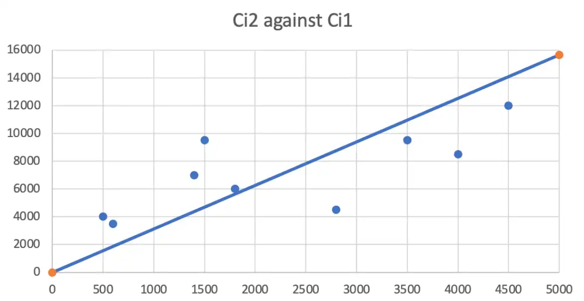
Underestimate losses less than 2000 and overestimate otherwise
- Mack suggest → Do a regression with an additional intercept parameter
If all pairings past the test, the dataset passes the test.

Spearman's rank Test (#1i¹)¶

KEYWORD = 'rank', which means we have to the =rank function ;)

Distribution free test for independence
Look at triangle as a whole (rather than individual pairs)

Looking at the whole triangle

Lets us know if correlation prevails globally than in a small part of the triangle.
Helps avoid an accumulation of error probabilities

\[ T_{k} \to 0 \implies \text{non-correlation} \]

Steps¶

Calculate LDFs
Rank the LDFs for each pair of factors
=rank(D1,D1:D3,1)

	$s_{i 2}$	$r_{i 2}$	$s_{i 3}$	$r_{i 3}$
$i=1$	2	1	1	2
$i=2$	3	2	2	1
$i=3$	1	3

Calculate $(r_{ik}- s_{ik})^{2}$ → sum column $S_{k}$

	$k=2$	$k=3$
$i=1$	1	1
$i=2$	1	1
$i=3$	$2^2=4$

Let $n$ be the number of Rank-pairs in column
$T_{k} = 1 - 6 \dfrac{S_{k}}{n(n^{2}-1)}$
$T$ = Weighted average of $T_{k}$ with $(\#AY-k-1)$ as weights

$k$	2	3
$T_{k}$	-0.5	1
$\text{weight}_{k}$	2	1

$E(T)= 0$ and $Var(T) = \dfrac{1}{(\text{\#AY}-2)(\text{\# AY}-3)/2}$
C.I. = $0 \pm z \sqrt{ Var(T) }$

Calendar Year Effects test (#2)¶

Reasons for calendar year effects

Internal
- Strengthening of case reserves
- Changes in claim settlement rates
External
- Legislative or legal changes
- Greater than average inflation

We fail to prove that there are significant calendar events.

Steps¶

Calculate LDFs
Calculate median
- $S$ → Smaller than median
- $*$ → equal to median
- $L$ → larger than median
Count $L$'s and $S$'s in each diagonal

$$
% Triangle Table
\begin{array}{c|cccc}
& j=1 & j=2 & j=3 & j=4 \ \hline
j=1 & L & \bbox[#B4B4FF, 2pt]{S} & \bbox[#FFFFC8, 2pt]{L} & \bbox[#B4F0B4, 2pt]{} \
j=2 & \bbox[#B4B4FF, 2pt]{L} & \bbox[#FFFFC8, 2pt]{} & \bbox[#B4F0B4, 2pt]{S} & \
j=3 & \bbox[#FFFFC8, 2pt]{S} & \bbox[#B4F0B4, 2pt]{L} & & \
j=4 & \bbox[#B4F0B4, 2pt]{S} & & & \
\end{array}

\[ \]

% Summary Table
\begin{array}{c|cc}
j & S_j & L_j \ \hline
2 & \bbox[#B4B4FF, 2pt]{1} & \bbox[#B4B4FF, 2pt]{1} \
3 & \bbox[#FFFFC8, 2pt]{1} & \bbox[#FFFFC8, 2pt]{1} \
4 & \bbox[#B4F0B4, 2pt]{2} & \bbox[#B4F0B4, 2pt]{1} \
\end{array}
$$

Step 4 (Znm) → "Zanam"
- $Z_{j} = \min(L_{j},S_{j})$ → Minimum
- $n_{j} = L_{j}+S_{j}$ → Addition
- $m_{j} =\text{rounddown}((n-1)/2,0)$
- $Z = \sum Z_{j}$
Step 5
- $E(Z_{j})=\dfrac{n}{2}-\binom{n-1}{m}\times \dfrac{n}{2^n}$
- $V(Z_{j})=\dfrac{n(n-1)}{4}-\binom{n-1}{m} \dfrac{n(n-1)}{2^n} + E(Z_{j}) - E(Z_{j})^{2}$

Then do hypothesis testing using this mean and variance. Just check if $Z=0$ appears in the 95% confidence interval (select $97.5$-th percentile since it is a symmetric interval)

Residual Plot Test (#3)¶

Plot the weighted residuals against $C_{ik}$
(CONSTANT VAR) $\propto 1$ → wtd. residual = $C_{i,k+1} - C_{ik}f_{k}$
(VAR PROP TO LOSS) $\propto C_{ik}$ → wtd. residual = $\dfrac{C_{i,k+1} - C_{ik}f_{k}}{\sqrt{ C_{ik} }}$
(VAR PROP TO LOSS$^{2}$) $\propto C_{ik}^{2}$ → wtd. residual = $\dfrac{C_{i,k+1} - C_{ik}f_{k}}{C_{ik}}$

Confidence Interval / MSE calculation¶

Deviation
$(\text{act}-\text{exp})^{2}$	k = 1	k = 2	k = 3	k = 4
i=1	0.000	0.003	0.000	0.000
i=2	0.029	0.001	0.000
i=3	0.003	0.002
i=4	0.003

Honestly, $k=1$ is not required. But may be required for $\alpha_{k}^{2}$ calculation

Master Table¶

k	1	2	3	4	5
alpha^2	4.46	2.24	0.00	0.00
alpha^2/f^2	2.37	1.52	0.00	0.00
dev i=4		765.00	928.79	1,123.72	1,172.58
inv sum		0.00181	0.00169	0.00176	0.00169

se(R)^2	3,777.84
Reserves	407.58

$\alpha^{2} = \dfrac{1}{(I-k-1)}\times \sum \prod(C_{k},\text{Deviations})$
inv sum = $\dfrac{1}{\text{Dev}}+ \dfrac{1}{\sum(\text{Col except Diagonal})}$
$se(R)^{2}=\text{Ult}^{2} \sum \prod(\dfrac{\alpha^{2}}{f^{2}},\text{inv sum})$

Interval Calculation¶

Since the reserves are following a log-normal distribution, the confidence interval can be found out like so:

$\sigma^{2}_{i} = \ln(1+ \dfrac{se(R_{i})^{2}}{R_{i}^{2}})$
CI = $R_{i} \times \exp(-\dfrac{\sigma^{2}_{i}}{2 }\pm z\sigma_{i})$

Muffs¶

Please read the entire question:
- On the top line one assumption was already given
- You were asked in (b) to give the other two. So, naturally you shouldn't state the one that was already mentioned before.

Implicit assumption: Development factors are not correlated ↩

Variance Assumptions	Dev factor, \(f_{k} =\)	Plain English
\(Var(C_{i,K+1} \\|\cdot)= \alpha_{k}^{2}\)	\(\dfrac{\sum_{i=1}^{I-k}C_{ik}^{2}f_{ik}}{\sum_{i=1}^{I-k}C_{ik}^{2}}\)	Constant variance, weight by \(C^2\)
\(Var(C_{i,K+1}\\|\cdot) = C_{ik}\alpha^{2}_{k}\)	\(\dfrac{\sum_{i=1}^{I-k}C_{ik}f_{ik}}{\sum_{i=1}^{I-k}C_{ik}}\)	Mack's case, weight by volume
\(Var(C_{i,K+1} \\|\cdot)= C_{ik}^{2}\alpha_{k}^{2}\)	\(\dfrac{\sum_{i=1}^{I-k}f_{ik}}{I - k}\)	Var prop to \(C^{2}\), simple average

	\(s_{i 2}\)	\(r_{i 2}\)	\(s_{i 3}\)	\(r_{i 3}\)
\(i=1\)	2	1	1	2
\(i=2\)	3	2	2	1
\(i=3\)	1	3

	\(k=2\)	\(k=3\)
\(i=1\)	1	1
\(i=2\)	1	1
\(i=3\)	\(2^2=4\)

\(k\)	2	3
\(T_{k}\)	-0.5	1
\(\text{weight}_{k}\)	2	1

Deviation
\((\text{act}-\text{exp})^{2}\)	k = 1	k = 2	k = 3	k = 4
i=1	0.000	0.003	0.000	0.000
i=2	0.029	0.001	0.000
i=3	0.003	0.002
i=4	0.003

Measuring the Variability of Chain Ladder Reserve Estimates - Mack (1994)

Study Strategy¶

Checklist¶

My Notes¶

Notation¶

Assumptions¶

Tests¶

Regression Test (#1)¶

Spearman's rank Test (#1i1)¶

Steps¶

Calendar Year Effects test (#2)¶

Steps¶

Residual Plot Test (#3)¶

Confidence Interval / MSE calculation¶

Master Table¶

Interval Calculation¶

Muffs¶

Spearman's rank Test (#1i¹)¶