Credibility
Three Necessary criteria
- Should be \(0 \leq Z \leq 1\)
- \(\dfrac{dZ}{dN} \gt 0\)
- \(\dfrac{d}{dn}(Z / n) \lt 0\)
Calculation
- Partial Credibility
- \(Z = \min\left(\sqrt{ \dfrac{n}{N_{0}} }, 1\right)\)
- Estimate = \(Z \times \text{Observed} + (1-Z) \times \text{Related}\)
- Buhlmann Credibility
- \(K = \dfrac{EPVP}{VHM}\) (Echoing/Valley)
- lower the expected Process variance \(\implies\) more homogenous (differences within the group are low) \(\implies\) more credibility
- More the variance between the the groups \(\implies\) more discrete clusters \(\implies\) more credibility
- Thus, small numerator, large denominator \(\implies\) small \(K\)
- \(Z = \dfrac{N}{N+K}\)
- Smaller the \(K\) \(\implies\) More the credibility
- Estimate = \(Z \times \text{Observed} + (1-Z) \times \text{Prior Mean}\)
- \(K = \dfrac{EPVP}{VHM}\) (Echoing/Valley)
- Bayesian Analysis
- Bayes Theorem
- Complex (unlikely to be tested)
Complement of Credibility
Six desirable qualities
- Accurate (close to target)
- Unbiased (=target, on average)
- Statistically Independent from base statistic (else errors compound)
- Available (else impractical)
- Easy to compute (else difficult to justify)
- Logical relationship to base statistic (else difficult to justify)
ABI, ACL: Abhi Asal mein…
Comparison of Credibility Complement Methods
This table evaluates five common methods for determining the complement of credibility against key actuarial criteria. A checkmark (✅) indicates the criterion is generally met, a cross (❌) indicates it is generally not met, and a question mark (❓) indicates it is conditional or variable.
| Method | Accurate | Unbiased | Independent | Available | Easy to Compute | Logical Relationship |
|---|---|---|---|---|---|---|
| Competitor's Rates | Biased if competitor makes different assumptions | Yes | Difficult to Obtain | Yes | Yes | |
| Loss Costs of a Larger Related Group | ❓ Possibly | ❌ Usually biased | ✅ Yes | ✅ Yes | ✅ Yes | ❓ If chosen reasonably |
| Loss Costs of a Larger Group (including subject) | ✅ Yes (due to stability) | ❌ Biased | ❌ No | ✅ Yes | ✅ Yes | ✅ Yes |
| Rate Changes from Larger Group Applied to Present Rates | ✅ Yes | ❓ Better (reduces bias of the above) | ❓ Yes, if subject data is excluded | ✅ Yes | ❓ Slightly harder | ✅ Yes |
| Harwayne's Method | ✅ Yes | ✅ Yes | ✅ Mostly | ✅ Yes | ❌ Harder | ✅ Yes (but harder to explain) |
| Trended Present Rates | ❓ Depends on the stability of indications | ✅ Yes | ❓ May or may not be | ✅ Yes (ALWAYS) | ✅ Yes | ✅ Yes |
- #Trended Present Rates is always available, if the company has written any policy in the past (as they need a rate to do it.)
Complements in First Dollar Ratemaking
Please note that the first 3 are are credibility weighting the LOSS COST! not the final indication.
LC: larger group including subject
- E.g. regional, countrywide etc
- Pros
- Accuracy (stability, larger data)
- Available
- Easy to compute
- May have logical connection
- Independent if subject experience excluded
- Cons
- Biased (there is a reason why subject group has been separated from larger group)
LC: larger related group
- neighbor
- Cons
- Biased
- Pros
- Available
- Independent
- Possibly accurate
- May have logical connection (if reasonably selected)
Rate changes from larger group applied to present rates
- Complement = Current LC of Subject \(\times \dfrac{\text{Larger Group Ind LC}}{\text{Larger Group Curr Avg LC}}\)
- Adjusted version of #LC larger related group to reduce bias
Harwayne's Method
This is for class ratemaking, not for overall indication.
Good problems
- Spring 2017 Exam 5 - Q9
Say we are trying to find a complement for State A, class 1
- Wtd Avg PP of State A
- Using State A's exposure distribution, Wtd Avg PP for B,C
- Adjustment factors \(\dfrac{\text{State A}}{\text{State B}}\) and \(\dfrac{\text{State A}}{\text{State C}}\)
- Adjusted PP
- State B, class 1 adjusted = SBC1 PP \(\times\) Adj Factor
- State C, class 1 adjusted = SCC1 PP \(\times\) Adj Factor
- Complement = average of adjusted PP, weighted on their exposure
Trended Present Rates
Use when there is no larger group.
- Accuracy depends on stability of (past) indications
- Unbiased (done by the actuary)
- May or may not be independent (done by the same actuary?)
- Readily available (apna hi company hai boss)
- Easy to compute
- Logical relationship to subject's experience (apna hi company hai boss)
Solve an example
| Variable | Value | Comment |
|---|---|---|
| Total Number of Claims in Historical Period | 3,612 | |
| Number of Claims for Full Credibility | 1,082 | |
| Credibility | 100.0% | Square root rule |
| Latest Indicated Rate Change | 13.2% | Calculated by the previous Actuary, not necessarily implemented |
| Last Rate Change Effective Date | 1/1/2016 | From [[One-time|On levelling Premiums]], last rate change date |
| Last Rate Change Taken | 5.0% | From [[One-time|On levelling Premiums]], last rate change |
| Residual Indication | 7.8% | The amount of change that couldn't be implemented. \(\dfrac{1.132}{1.05}-1\) |
| Projected Loss Trend | 0.5% | From Loss trending |
| Projected Premium Trend | 2.0% | From premium trending |
| Net Trend | -1.5% | The loss ratio trend |
| Trend Period | 1.0 | From last rate Change effective date to the future effective date in quesiton. |
| Trended Present Rates Indication | 6.2% | Project the residual indication to the future. =(1+B15)*(1+B19)^B21-1 |
Pure Premium Method
Hands-on explanation. Take this example
| $200 | Present average rate |
|---|---|
| 10% | Annual loss trend |
| 20% | Rate change requested in last filing |
| 15% | Rate change approved with last filing |
| January 1, 2006 | Effective date requested in last filing |
| June 1, 2006 | Actual effective date of last change |
| January 1, 2008 | Proposed effective date of next change |
- We need to calculate the complement of credibility using trended present rates approach.
- What are we trying to find now?
What would be the present rate had the requested rate filing, WOULD HAVE BEEN APPROVED NOW?
- The actuary 2 years ago, would have calculated on Jan 1, 2006, that the rate change should be 20%
- But after some implementation protocol, they approved 15% rate change.
- Let's look at the solution and break down the answer for ourselves
=B8*(1+B10)/(1+B11)*(1+B9)^2
- We are adjusting the \(\text{Present Avg Rate}\)
- By removing the effect of the \(\text{Aproved RL chg}\) and applying the \(\text{Requested RL chg}\) to it, this takes care of the part "HAD THE requested rate BE APPROVED NOW".
- Apply the \(\text{Loss Trend}\) because times have changed.
- The \(\text{Trend Period}\) would be:
- From: The date for which the previous actuary actually performed the calculation
- To: The future policy period when the rates will be in effect.
- Hence, it should be 2 years (Jan 1, 2006 \(\to\) Jan 1, 2008)
Calculation:
Loss Ratio method
- Basically, undo the effect of implementation
- Apply the actual calculation…
Complements in Excess Ratemaking
Complement when estimating excess losses.
NOTE: These are complements of losses. If you are asked to find the complement of loss cost in the question, then ensure that you divide it by earned exposures before submitting your answer. Give what is asked for!
- Estimate of losses
- Estimate of loss cost
Increased Limits Analysis
When ground-up loss data up to attachment point, \(A\) is available.
For \(L\text{ xs }A\),
- Dividing by \(ILF_{A}\), makes losses capped to basic limit
- Then we multiply by the differential that lets us know the losses in the layer L xs A
So, essentially it is,
Note the distinction between actual and expected in the formula above.
- Notes
- If expected values come from a different size of loss distribution than subject experience
- \(\implies\) Biased complement
- If data available \(\implies\) Independent and practical
- but biased
- inaccurate due to low volume of data
- If expected values come from a different size of loss distribution than subject experience
Lower Limits Analysis
Use data at a lower limit \(d\) than the attachment point, \(A\). \(d \lt A\)
Intuitively,
so, using \(ILF\)s,
- more bias, but also more accuracy
Limits Analysis
Further generalization of #Increased Limits Analysis
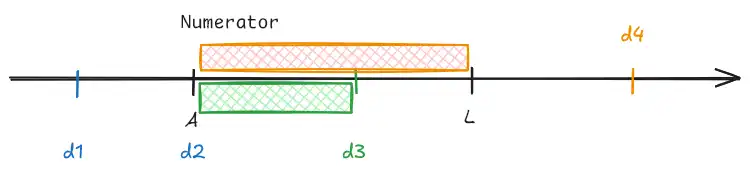
| Limit | Contribution to complement | |
|---|---|---|
| \(d_{1}\) | Doesn't contribute | so \(d\geq A\) |
| \(d_{2}\) | \(ILF_{A}- ILF_{A}=0\) | so \(d\gt A\) |
| \(d_{3}\) | \(\dfrac{ILF_{d_{3}}-ILF_{A}}{ILF_{d_{3}}} \times E(\text{Loss capped }d_{3})\) | \(\checkmark\) |
| \(d_{4}\) | \(\sum_{d_{4}\gt A+L} \dfrac{ILF_{A+L} - ILF_{A}}{ILF_{d_{4}}}\times\) \(E(\text{Loss capped }d_{4})\) | Just like #Increased Limits Analysis but allows data from higher limits. |
- Biased and inaccurate
- Assumes loss ratio doesn't vary by limit
- Used by reinsurers who don't have ground-up loss data