One-time changes
Workers Compensation Benefit Change
Intuition
For SAWW problem think of the limits like so
- Remember Benefit = Claim
- If problem stated in percentages, a simple mental model
- Avg Wage in Rage (not required to calculate)
- % wage = \(\dfrac{W}{TW}\)
- % workers = \(\dfrac{\#}{T\#}\)
- So, \(\dfrac{\%\text{wage}}{\%workers}\) = \(\dfrac{\frac{W}{TW}}{\frac{\#}{T\#}} = \dfrac{\frac{W}{\#}}{\frac{T\#}{TW}} = \dfrac{\frac{W}{\#}}{SAWW}\)
- Get the Avg Benefit/SAWW \(\to\)
SUMPRODUCTwith %workers to get Avg Benefit of total/SAWW- (min) \(\dfrac{\text{Avg Benefit}_{1}}{\text{SAWW}}, \dfrac{\text{Avg Benefit}_{2}}{\text{SAWW}}, \dots\)
- (in range) \(\dfrac{\frac{W}{\#}\times \frac{2}{3}}{\text{SAWW}}, \dots\)
- (max) \(\dots,\dfrac{\text{Avg Benefit}_{n}}{\text{SAWW}}\)
- Then do
SUMPRODUCTwith %workers, only \(\text{Total Benefit in Range}_{i}\) and \(W \times \dfrac{2}{3}\) will remain in the numerator, and \(SAWW \times T\#\) in the denominator- Because remember, %workers = \(\dfrac{\#}{T\#}\), when multiplied to each term, the \(\#\) cancels out but the \(T\#\) remains…
- So you get \(\dfrac{\frac{\text{Total Benefit}}{T\#}}{SAWW}\) and when comparing current and proposed, the \(SAWW\) cancels out.
- Compensation rate = \(\frac{1}{2}\) (say)
- For an individual % to average weekly wage = \(X\) (say)
- @Current Rates (min = 50% and max = 125%, say)
- Minimum is applied when \(X \times \frac{1}{2} \leq 50\%\) (i.e. minimum)
- Solving for which we get \(X \leq \dfrac{50\%}{\frac{1}{2}} = 100\%\)
- So, when it is \(100\%\) or below
- Minimum is applied when \(X \times \frac{1}{2} \geq 125\%\) (i.e. minimum)
- Solving for which we get \(X \leq \dfrac{125\%}{\frac{1}{2}} = 250\%\)
- So, when it is \(250\%\) or above
- Minimum is applied when \(X \times \frac{1}{2} \leq 50\%\) (i.e. minimum)
- Do the same for revised rates, the logic for dividing the min and max by the compensation rate to find the critical point, is the main crux of this discussion and now should be clear.
- Avg Wage in Rage (not required to calculate)
Table
| Received | by | +/- | ||
|---|---|---|---|---|
| Current | Min | $550.0 | 100% | or below |
| Max | - | - | ||
| Comp rate | 1/2 | |||
| Revised | Min | $550.0 | 75% | or below |
| Max | $1,375.00 | 187.5% | or above | |
| Comp rate | 2/3 | |||
| ## One-time Premium Changes |
Extension of Exposures
- Extension of exposure method
- re-rates all policies written in the historical period using the current rates. \(\implies\) More accurate ✅
- Problematic if a new rating variable is introduced \(\impliedby\) there might not be historical data available related to those variables
- Requires more detailed data for each policy & more time to calculate.
- Parallelogram method
- Simpler, no detailed data required. ✅
- Need overall-rate changes and historical earned premiums to on-level premiums.
- Much less accurate than EOE & less reliable when used in classification ratemaking
- Solution: Capture rate changes at the class level and use parallelogram method at a class level instead of aggregate
- Assumes, policies have been written uniformly over time \(\implies\) inaccurate on-level premiums if assumption doesn't hold.
- Solution 1: Smaller time periods
- Solution 2: #Actual Writings Distributions & Group Data by RL
Parallelogram Method
- For Parallelogram method, ensure:
- annual or semi-annual policies...
- This should be the format to calculate portion: \(\dfrac{1}{2}\times \dfrac{\text{\# months}}{12} \times \dfrac{\text{\# months}}{6}\) where:
- \(12:\) number of months in CY
- \(6:\) total number of months for a single policy.
- In case of uneven exposures writing you need to calculate the following
- Average Date (from before the CY and during the CY)
- % written (given as the distribution)
- % earned in CY 2014 (one we are interested in)
- Here we are talking about, how much of that chunk (corresponding to the average date) was earned in CY 2014
- % of CY 2014 earned
- Here, we are talking about, how much of CY 2014 was earned due to that chunk.
- Please note the difference between the above two.
- Proceed with usual average rate level calculations
Calculating areas of geometric shape
- Just do, \(\dfrac{1}{2} \times \dfrac{\#\text{months}}{\text{6-month policy}} \times \dfrac{\text{\#months}}{3 \text{(if CQ/PQ)}}\)
- 3 = 12/4, i.e. each quarter has 3 months \(\implies\) numerator and denominator matches. 6 = 12/2 for semi-years, 12 for annual.
Uneven exposures
- Parallelogram method won't work directly, but we can make it work!
- Just remember, the trick lies in finding out the average rate level of a particular aggregation (year).
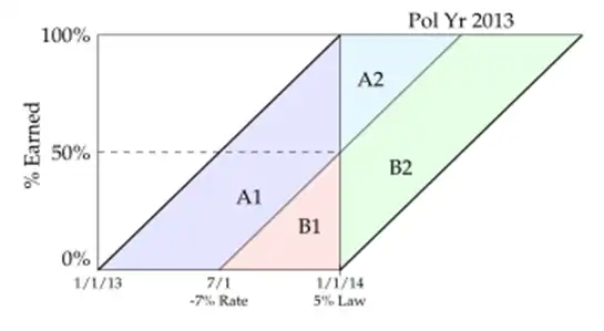
- For example, if 1/1/13 to 7/1/13 had 10 exposures per month. But 7/1/13 to 1/1/14 have 11 exposures per month.
- Then we just need to find the average rate level
- by recognizing that A1+A2 level should get \(\dfrac{10}{12}\) weight, while B1+B2 should get \(\dfrac{11}{21}\) weight.
- Suppose average rate levels are given as
| Area | Rate Level |
|---|---|
| A1 | 1 |
| A2 | 1.05 |
| B1 | 0.93 |
| B2 | 0.977 |
Then our average rate level for PY2013 is:
For a better understanding, see what we would get if exposures were even
Notice the weights,
| Area | Portion for even exposures | Portion for uneven exposures |
|---|---|---|
| A1 | \(75\% \times \dfrac{10}{20} = 37.5\%\) | \(75\% \times \dfrac{10}{21} = 35.71\%\) |
| A2 | \(25\% \times \dfrac{10}{20}=12.5\%\) | \(25\% \times \dfrac{10}{20}=11.90\%\) |
| B1 | \(25\% \times \dfrac{10}{20} = 12.5\%\) | \(25\% \times \dfrac{10}{20} = 13.10\%\) |
| B2 | \(75\% \times \dfrac{10}{20} = 37.5\%\) | \(75\% \times \dfrac{10}{20} = 39.29\%\) |
CY WP without Law changes
For CY WP (without Law changes), we just need to find the portion of policies written at each rate level
- (e.g. if \(+10\%\) rate change at July 1, 2025. Then OLF for CY 2025 would be \(1\times 0.5 + 1.10 \times 0.5\))
CY WP with Law changes
For CY WP (with Law changes), the process is a little involved.1
Answer the question:
What is the total Premium written in CY 20xx?
- Say, we have the rate changes:
- 4/1/12: +10% (experience)
- 7/1/12: +5% (law change)
- Partition the CY into segments between the rate changes, and under the assumption (100 policies per year, and 1000 per policy, before rate change)) find the premium written in that year, appropriately.
- Next, find how much does the law change contribute to the increase in total premium written for in-force policies (so, don't double count the premiums calculated in the previous step)
- Starting from the first date, from which policies are affected by the law change (10/1/11), till the first experience rate change (3/31/12). This is the first portion we will inspect. 50 policies will be written in this rate (6 months \(\times\) 100 per year = 50)
- The average date for this portion is 1/1/12. So, the average policy will have 3 months remaining after the law change on 10/1/12 (i.e. 3months between 10/1/12 \(\to\) 12/31/12)
- So, the contribution from this would be \(50 \times \dfrac{3}{12} \times (1000 \times 5\%) = 625\)
- Similarly, from the portion, 4/1/12 \(\to\) 9/30/12, the contribution would be \(50 \times \dfrac{9}{12} (1100 \times 5\%)=2062.5\) (since, post 4/1/12, the rate would be 1100 per policy and 9 month on average would be left for each policy after the LC)
- Now, answer the first question. Sum all these and get CY 2012 WP .
- To obtain the answer
If you understood this much then this diagram should be enough to remember the entire story
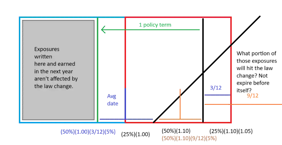
- Avg Rate Level:
sum- \((25\%)(1.00)+(50\%)(1.10)+(25\%)(1.10)(1.05)\) ← Written on the same year
- \(+ (50\%)(1.00)\left(\dfrac{3}{12}\right)(5\%) + (50\%)(1.10)\left(\dfrac{9}{12}\right)(5\%)\) ← Written on previous year
- \(=1.1156\)
- Current Rate Level:
- \((1.00)(1.10)(1.05)= 1.155\)
- On-level Factor
- \(\dfrac{1.155}{1.1156}=1.0353\)
Actual Writings Distributions & Group Data by RL
- Rate change: +5% on Sept 1, 2014
- Find CY2014 EP OLF
| Quarter | Written Exposures |
|---|---|
| 2014 Q1 | 100 |
| 2014 Q2 | 300 |
| 2014 Q3 | 500 |
| 2014 Q4 | 700 |
- Flow
- Written Exposures (group by RL)
- RL for each group
- Average written Date (find)
- %earned for the CY (for which you wish to find the OLF)
- You can make as many as you want
- CY earned exposures
| Quarter | Writ Exp | RL | Avg Writ Date | %earned in CY 2014 | CY 2014 Earned Exposures |
|---|---|---|---|---|---|
| 2014Q1 | 100 | 1 | 2/15/2014 | 0.878 | 87.78 |
| 2014Q2 | 300 | 1 | 5/15/2014 | 0.628 | 188.33 |
| July+August | 333 | 1 | 8/1/2014 | 0.417 | 138.89 |
| September | 167 | 1.05 | 9/15/2014 | 0.294 | 49.07 |
| 2014Q4 | 700 | 1.05 | 11/15/2014 | 0.128 | 89.44 |
| 12/31/2014 |
-
Use
yearfrac()to quickly find the % earned (only works for annual seamlessly), but think a bit for non-annual policies (semi-annual, multiply by 2 andmin(1,...)) -
CY2014 Avg Earned RL =
sumproduct(CY2014 Earned Exposures, RL) - OLF = \(\dfrac{\text{Latest}}{\text{Avg RL}}\)
Direct & Indirect Effects
- Direct and obvious impacts to premiums, losses or expenses solely due to the change, all else being equal, not taking into account the human response to the change.
- Indirect effects (aka incentives) are impacts to premiums, losses or expenses that arise due to changes in human behavior that are consequences of the one-time change.
- e.g. Increase in the maximum benefit make Workers stay out of work for longer due to the increased financial incentive. (Duration)
- e.g. More benefits are filed for due to the increased financial incentive (Frequency)
- A #tip, give examples when answering such questions, where even you are unsatisfied with your verbose explanation.
Complex problem strategies
- (Theory) Strategies for detailed non-uniform exposures
- Find the % of CY earned from % written and % of chunk written in CY
- Extension of exposures method
- Parallelogram method on a quarterly basis
Misc
- Wording
- Effective through (means till that point in time)
- Effective from (from that point in time)
- Loss Ratio method \(\to\) We are dealing with Premiums #doubt (Fall 2018, Q3(c))
- On-levelling for losses
- Estimated reduction to ultimate claims based on law change effective July 1, 2012, applicable to all claims occurring after the effective date \(\implies\) We have to treat it like a 50-50 law change. So, draw the lines straight and not like a policy year wise. #doubt Why straight lines?
- Remember: the following are equivalent in terms of process
- On-levelling CY Earned Premium
- On-levelling PY Written Premium
- Note that EP of a PY is same as the WP. (or For PY, \(EP = WP\))
-
The complexity arises from the fact that policies written before the PY even started, but since the law change happened during the PY in question, the extra premium from that would be associated with not the previous PY, but the current one. For example, if we are looking at PY 2025, and there was a law change of +5% on July 1, 2025… then some policies written in 2024 have to get revised if they are in-force during July 1. In such a case, the extra premium of 5% \(\times 1000 = 50\) will be part of PY 2025, and we have to account for that in our calculation. ↩