Careful
Don't Waste Time
For Pure Premium approach for indication.
Since we need to calculate the indicated rate and not an indicated rate change, all the premium info including the premium trend is irrelevant to this question.
Don't make repeat mistakes
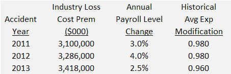
Here, annual payroll level change should be interpreted as: 2.5% from 2012 to 2013 (the value is for the to-year). \(=\dfrac{\text{Current}}{\text{Previous}}\)
A claims-made policy should always cost less than or equal to an occurrence policy.
- Is this statement true?
- No… look out for the keyword always, CM policy costs less only if the claim costs are increasing.
| Year Ending Quarter - X | Written Premium at CRL | Written Exposure |
|---|---|---|
| 2010 - 2 | $1,314,117 | 12,752 |
| 2010 - 3 | $1,323,381 | 12,776 |
| 2010 - 4 | $1,333,726 | 12,806 |
| 2011 - 1 | $1,343,014 | 12,825 |
| 2011 - 2 | $1,354,391 | 12,863 |
Year Ending quarter refers to a full year, thus when you are selecting trend periods from this, you should ensure that you are considering sa 12 month period and not a 3 month period (quarter) just because its written in quarters.
So, midpoint of year ending quarter 2010-4 = 7/1/2010
Don't forget to multiply the tail factor appropriately. Messes up the calculation otherwise, made an error while going through the Appendices
STRIKE 2: Practice exam 1
You forgot to multiply the tail factor again! Q19
Trend dates for:
- Exposures \(\to\) Earned
Suppose an adjustment factor (1.05) applies to only 40% of the element (loss/premium) you are trending. For the rest, the adjustment is (1.10)
Let the loss/premium be $100,000. Then, the correct projected amount would be:
To find the combined effect in a single factor to be applied to the premium $100,000.
The combined factor is
- Thus, we have to weight, the adjustment factor and NOT the percentage value, in order to get the correct combined effect.
If multiple years are given, sum the averages of each category of expense… i.e. Avg Gen Expenses + Avg Other Acquisition + Avg Licenses & Fees. instead of taking the average of 2012 and 2013 expenses. Though it results in the same output. but always good to take the average at a more granular level
- Policies are annual
Look at this statement about a law change:
Law change requiring the insurer to pay for diminution of value was implemented 4/1/2013 and change affected losses on policies written on or after implementation date. Estimated increase in losses due to change is 10%.
- NOTE: losses on policies written on or after implementation date.
- So, if we use this fact to on-level our loss our diagram should look like this
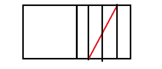
- So our on-level factors for each quarter in 2013 would be
- 2013Q1 = \(1.10\)
- 2013Q2 = \(\dfrac{1.10}{1\times(0.75) + 1.10 \times(0.25)}\)
- 2013Q3 = \(\dfrac{1.10}{1\times(0.25) + 1.10 \times(0.75)}\)
- 2013Q4 = \(1.0\)
Vertical line when the tort reform affects all accidents after the law change.
When calculating rate for an ITV problem. It will be per "Rate per $ of coverage for 80% ITV", so you should remember to divide by \(80\%\).
STRIKE 2: Practice exam 2
Again, for an ITV problem. You were asked to find the rate per $100 of insured value (you divided it by the property value instead! Don't do that bro!)
- Divide by coverage amount and NOT the replacement amt.
Trended Present rates: the trend period is from ORIGINAL EFFECTIVE DATE (not some average earned/written date). It's between effective dates! Please remember that.
To determine the trends from quarterly premium data, you must use Average on-leveled premiums because:
- we want to isolate the effect of exposure differences across periods \(\to\) Average
- we want to isolate the effect of one-time premiums for calculating our trends \(\to\) On-leveled
And also, just because more granular data is given in the question, don't feel obligated to use it. For example, if quarterly not-leveled average premiums are given, then you have to take another step to on-level them and calculate the premium trends.
Instead, if you have already calculated on-leveled premium and have exposure information then feel free to use it! Nothing wrong!
For non-modeled cat-loss loading, we need to find the Average AOI per exposure that corresponds with the future average EARNED date. For that we must interpolate between the average AOI's given such that we achieve the value corresponding to the future average earned date. E.g.
- We have CY2015 (Avg AOI = 272.8) and CY2016 (Avg AOI = 280.99)
- Our required future average earned date = 1/1/2016
- Average CY2015 (7/1/2015) and CY2016 (7/1/2016) to get the value
Commissions are 100% variable, if not mentioned, ensure you put entire of it in Variable expenses and none of it in fixed expenses. There was an instance when you left it out in both!
You are not paying attention to on-leveling written premium, always performing the earned strategy. Be mindful!
When asked to find the incremental triangle for 2012 - 2015, ensure that you include rows for all years AY12, AY13, AY14, AY15 (even if AY14 and AY15 have zero values)
While creating incremental triangles, ensure that you are considering the claim numbers to get the change in case reserves right.
When talking about why trending should be done on on-leveled data. You should not just say one-time changes, you should also mention rate-changes since that is the one-time change on premiums that we do.
When asked about effect on average premium due to a rate change, you should mention (ideally both) the direct and indirect effects.
Ensure to check what is the basis of the credibility calculation, is it claim counts? or is it exposures?
When credibility weighting in Loss Ratio Approach, don't be overconfident. If you are weighting the Factor change, \(C=1\), if you are weighting the % change, \(C=0\).
Don't use the shortcut formula for Benktander method, in order to find unpaid/IBNR. Calculate the IBNR manually only
When trying to find the rate change factor for each of the relativities, multiply also by the OBF (you are looking at the % change in premiums, not just relativities) only when Additive fee = 0
If additive fee is not zero, then we need to find the average premium using the rating algorithm that includes the additive fee and then compare the premiums.