Trends
- ASOP 13 (Trending)
- 4 sections to be read… section 3 most relevant
- 2.6 - ASOP 13 applies to all kinds of trends
- Not just premiums and losses
- expenses, retention rates, marketing response rates too
- 3.1 - Presentation
- Point estimate vs Range of estimates
- Intended purpose
- How to calculate?
- How to present?
- 3.2 - Data
- Insurance (Fast Track) or non-insurance (economic CPI)
- Credibility
- Time period of available data (realization)
- relationship of data to what is being trended6
- any known distortions in the data
- seasonality
- change in practices
- change in mix of business
- impact of catastrophes
- 3.3 - Consider relevant social/economic influences
- e.g. claim consciousness, court practices, legal precedents
- 3.4 - Selection of the procedure
- Current best practices
- Methods used in prior analysis
-
The fundamentals of trending
-
(Theory answers)
- Why we trend in rate level indication?
Adjust for premium differences between historical and future periods based on things like changing mix-of-business and socio-economic trends/conditions - Why we don't use historical premiums?
Because one-time rate level changes would be picked up by the determined trend, though we don't expect these one-time changes to continue in the future. - When can we observe negative (positive) average premium trend?
- Insureds moving to higher (lower) deductibles
- Insureds buying lesser (more) coverage
- Insurer writing more low- (high-) risk policies
- Insurer might be non-renewing high- (low-) risk policies5
- Why we shouldn't use XS/Total trend for basic limits ?
Because the Total trend would ignore that the basic limits losses cannot exceed the basic limit.
- Why we trend in rate level indication?
-
We are not concerned with the total number of policies that the insurer will write in the future. Total number of policies will determine the size of the business, we are not trying to see how the size of the business grows or shrinks
- We are trying to see how the average costs and average premiums change over time.
- Due to various reasons
- Change in the general price level (inflation) \(\implies\) Payroll increases \(\implies\) Exposures of workers comp increases.
- Rise in gas price \(\implies\) less cars driven \(\implies\) lower Frequency of accidents
- Increase in cost of medicines \(\implies\) increased claim Severity.
- Historical on-leveled premium data will be adjusted to the future level by applying the premium trend. \(\impliedby\) On-leveling is done before the application of the trend.
- \(\lvert \text{Basic Loss Trends} \rvert \lt \lvert \text{Excess Trends} \rvert\)
- Which means basic loss trends are closer to zero than the excess trends (also, total trends)
- Reason:
- For losses, above basic limits… the trend1 is in the entirely in the excess layer
- Losses just under the basic limits, get pushed into the excess layer by trend \(\implies\) creating newer losses for the excess layer.
- Exception:
- Loss trends are negative: Basic loss trend will be closer to zero and the XS loss trends will be more negative.
- Trend period simplifying assumptions \(\implies\) Use average dates to represent each group of data2
- Policies are written uniformly over time
- Premiums are earned uniformly and claims occur uniformly over the policy period.
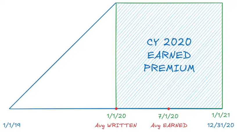
- Mental model for dates
- Look at CY 2020 EP
-
WP contributing to it: 1/1/2019 \(\to\) 12/31/2020
- Midpoint = 1/1/2020 (Avg Written Date)
-
These written policies will earn: 1/1/2019 \(\to\) 12/31/2021
- Midpoint = 7/1/2020 (Avg Earned Date)
- General formula for CY YYYY
- Avg Earned Date = 7/1/YYYY
- Avg Written Date = 7/1/YYYY \(-\) Half the policy length
Premium is written first and then earned (midpoint) \(\implies\) Written is before midpoint.
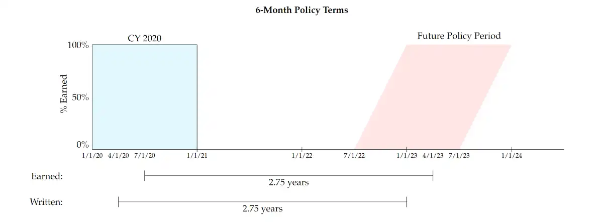
- Two step trending
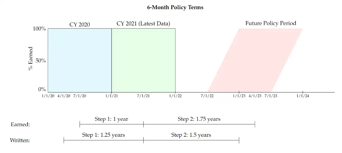
- Historical Period (Historical trends)
- Hist date: Earned (or written = earned - half)
- Latest Average Written/earned date: (Earned = Written) date (midpoint)3
- Future Period (Prospective trend)
- Future average earned/written date: based on formula
- Note: Future "Policy" Period (see figure below)
- Why or when is it appropriate? "When historical trends are expected to be different from the prospective trends."
- e.g. Temporary shifts in the policy limits in the historical period
- Advantage: Allows for different trends to be taken in experience period and from experience period to
- Note the relationship between written \(\to\) earned
- Note the difference between:
- Policy term: A duration for a single policy
- Rate revision (Policy Period): The duration in which rates will be in effect (Policy Period that we refer to) \(\impliedby\) We have to take the average earned/written dates of this policy period (can be 12 months) and NOT policy term (can be 6 months)
- \(\implies\) We only take average dates of AGGREGATION PERIODS (CY/PY) and NOT POLICY TERMS
- Two step trending (with exposures given)
- \(\text{Trended OLEP}\) =
- \(\text{Hist. OLEP} \times \dfrac{\text{Latest Avg OLWP}}{\text{Hist. Avg OLWP}}\times \text{Step 2 trend}\)
- \((\cancel{\text{Hist. Avg OLEP}}\times \text{Hist. EE} )\times \dfrac{\text{Latest Avg OLWP}}{\cancel{\text{Hist. Avg OLWP}}}\times\dots\)
- \(\text{Hist. EE} \times \text{Latest Avg OLWP} \times \text{Step 2 trend}\)
- Use OLWP whenever possible… more recent. #doubt (logic)
- Step 1 trend factor = \(\boxed{\dfrac{\text{Latest Avg OLWP}}{\text{Hist. Avg OLEP}}}\)
-
CY Average Earned Prem @CRL Average Written Prem @CRL 2009 $375 $380 2010 $390 $395 - Say the above is given, then still we need to find the Step 1 trend factor even for CY 2010 as \(\dfrac{395}{390}\) even though theoretically it should be \(1\)… because remember, we are comparing written to earned so there will be a slight difference that can be accounted for using this factor.
- (Two step) Trending for losses
- Here we are dealing with Accident Years \(\implies\) Use Average Accident Dates
- Future policy period \(\implies\) Average written date. For example, for the policy period: 7/1/2013 \(\to\) 7/1/2014, the average written date: 1/1/2014
- Thus, an average policy will be written on 1/1/2014. Thus, the average accident date of this policy would be: 1/1/2014 \(+\) Half the policy length = 7/1/2014
- Note that this is the same as Average earned date (which is logically consistent4)
- Calculation of Trend Rates
- You only trend Premiums @CRL: First on-level your premiums, then use them to calculate the trends, the trends shouldn't reflect rate changes… Look at rate changes as one-time abrupt changes that can be accounted for by "re-stating historical premiums at the current rate levels."… We don't expect these ONE-TIME changes to continue in the future
- Trends that show up in Written Premium will eventually show up in Earned Premium.
- Selecting trend rate from Exponential fits
- Wording
- 12 months ending each quarter refers to Calendar years, so the trend rates are actually annual.
- Spring 2015 Q4: Pick something that is minimally influenced by the deductible shift is the key. Deductible shift impacts policies renewing as late as 6/31/2012, which would earn as late as 6/31/2013, so select # of points that do not include dates till 6/31/2013 (here 6 points) \(\implies\) Select 4 point or 6 point average
- Fall 2015 Q4: Picking 2 step trending for frequency, since it shows a structural change midway and we are finding a pure premium trend factor for CY 2012 which appears to be before the structural change.
- Fundamental #doubt, how does this exponential fitting actually work
- Wording
- Loss cost = Pure Premium
- AQ 2014Q4: Fourth Accident quarter of year 2014
- Experience period: Historical period to latest period
- Future Policy period: Policy effective period.
- Model year and symbols rating plan #doubt
- You can also state 2-step trend periods as
- Date 1 to Date 2 to Date 3
- Instead of
- Step 1 trend period: …
- Step 2 trend period: …
- On-levelling loss data
- "Policies on or after … have a +10% benefit change" \(\to\) Experience
- "Accidents occurring on or after… have a +10% benefit change" \(\to\) Law change
- Misc.
- If we assume that fixed expenses and premiums are trending at the same rate then we don't need to apply trends to fixed expense ratio.
- Say, you are pricing deductible policies BELOW the indicated rates to incentivize the policyholders to move to a higher deductible.
- Indicated rates are set so that the insured can cover off all the expected costs and also be able to meet the target profit. But, in this case the policies are priced below the indicated rate. Thus the decrease in deductibles as a result of policyholders moving to a larger deductible higher than the decrease in the expected claims due to that deductible. Hence, the profitability will reduce.
- If a change,
- for example
- lower number of high deductible policies written
- change in UW guidelines that lead to a reduction in the claim counts.
- isn't reflected is not reflected in the trend data yet, then we can say that the estimate for our trended result (whatever it may be, loss etc) has to change (should be higher/lower).
- for example
-
-
Substitute trend for "increase/decrease" in value ↩
-
This is why we are able to take average dates, these assumptions allow us to do so. ↩
-
Why is earned and written date the same? Suppose the historical period is given as 1/1/2001 to 12/31/2003. In these three years, the last year i.e. CY 2003 will be considered the l "latest average written (or earned) date". The written date is straightforward, the midpoint. The earned date (owing to the assumptions) will also be the midpoint, since it is coming from policies written in CY 2002 and CY 2003. So, it fills the CY 2003, like a full square instead of a half triangle as far as earning is concerned. ↩
-
Think of exposure to accidents and earning of premiums as two sides of the same coin. "An individual is exposed to risk, but he transfers that exposures by paying a commensurate amount of money to the insurer for that time period. The amount that the insurer earned for that time period is called earned premium." Thus, the average accident date and the average earned date are really the same thing, if we talk about the same policy period. ↩
-
However, the non-renewing low risk policies (in the brackets) doesn't make sense. Why would you do that? ↩
-
E.g. if we are trending pure premium, we are trending losses ↩