Diagnostic Checking
- We did L16__Model Identification and L17__Model Estimation. Now we need to
- check the goodness of fit
- check the validity of assumptions (on errors)
- Then do forecasting
Normality of Errors
-
How to check if the errors are normal?
- Check the histogram of the standardized residual, \(\dfrac{\hat{e}_{t}}{\sigma_{e}^{2}}\)
- Draw normal Q-Q plots
- Look at Tukey's "five number summary" to check for normality
- Skewness = 0?
- Kurtosis = 3?
- Excess kurtosis = 0?
- Hypothesis tests
- Shapiro-Wilk
- Jarque-Bera
-
If the sample size is relatively small, then the simulated distribution will be skewed even if it is drawn from a normal distribution.
Jarque-Bera Test
- Tests whether skewness or excess kurtosis are collectively equal to 0 or not?
- \(\beta_{1}\) = skewness
- \(\beta_{2}\) = kurtosis
\[
JB = \dfrac{n}{2} \left[ \beta_{1}^{2} + \dfrac{(\hat{\beta}_{2}- 3)^{2}}{4}\right] \sim \chi_{2}^{2}
\]
The Hypothesis Setup
\[
\begin{matrix}
H_{0} : & \text{Normality} \\
H_{\alpha} : & \text{Non-Normality}
\end{matrix}
\]
Shapiro Wilk Test
\[
W = \dfrac{\left( \sum_{i=1}^n a_{i}x_{(i)} \right)^{2}}{\sum(x_{i}- \bar{x})^{2}}
\]
where,
- \(a_{i}\) are constants
- \(x_{(i)}\) denote order statistics.
Reject normality if \(W\) is too small.
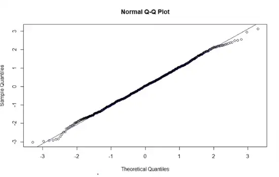
Normal Q-Q Plots
- 95th quantile (95% of the values are smaller than this 95% quantile)
- X-axis: Theoretical quantiles (assuming standard normal distribution)
- Y-axis: Actual quantiles from the sample distribution.
If the graph shows a straight line then normality holds true.
Normality holds:
Normality doesn't hold:
Detection of Serial Correlation
"Serial autocorrelation": Residuals are found to be correlated with their own lagged values.
Draw the ACF plot:
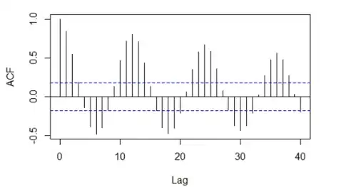
If there is this kind of pattern in correlations, we can say that there is serial autocorrelation (current error and one error in the future and the past are correlated).
Box-Pierce Test
\[
H_{0}: \text{data are independent (no correlation)}
\]
\(h\) is the number of lags up to which we would check for.
-
\[ Q_{BP} = n \sum_{k=1}^h \hat{\rho}_{k}^{2} \]
If \(Q_{BP} \gt \chi_{1-\alpha,2}^2\)
- reject null \(\implies\) Autocorrelation in residuals
- recheck model → Better add another lag in either AR or MA part of the model.
Ljung-Box Modified Test
- \(n\) is the sample size, \(h\) is the number of lags being tested
- Mostly same as #Box-Pierce Test
- Modified by Ljung and Box in 1978.
- \(n^{2}\) and \(n-k\) in denominator
\[
Q_{LB} = n^{2} \sum_{k=1}^h \dfrac{\hat{\rho}_{k}^{2}}{n-k}
\]