Cyclicity and test for Stationarity
- Cyclical variations
- gradual, long-term, up-and-down irregular repetitive movements
- rise and fall are not of fixed frequency
- period usually extends beyond a single year
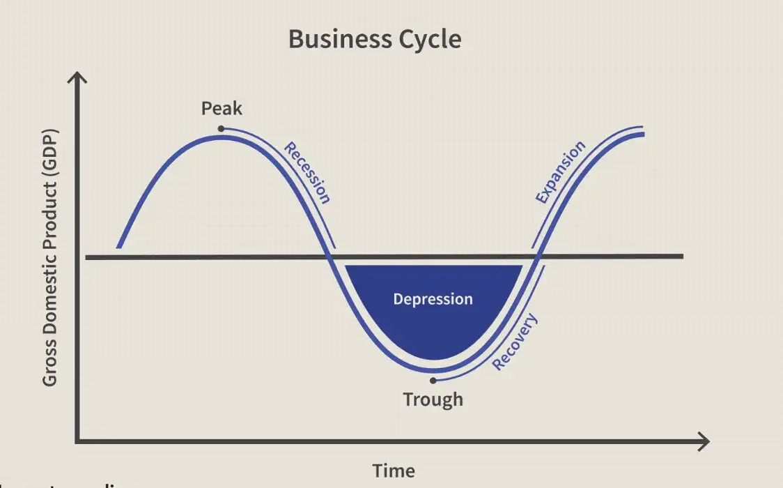
- 6 phases (Business Cycle)
- Expansion
- Peak
- Recession
- Depression
- Trough
- Recovery
- Examples
- Business cycle
- Price cycle : production decision
- Solar cycle: Sun's magnetic field (every 11 years, Sun's north and south poles shift entirely)
| Seasonality | Cyclicality |
|---|---|
| Calendar Efffects | Fluctuations not of fixed frequency |
| Average length is smaller | |
| Magnitude of cycles are higher |
Unit Roots
\[
Y_{t} - 1.9 Y_{t-1} + 0.9 Y_{t-2} = e_{t} - 0.5 e_{t-1}
\]
can be REwritten as
\[
(1- 1.9B + 0.9B^{2}) Y_{t}
\]
The roots of this equation are \(1\) and \(\dfrac{10}{9}\). Thus, this model has a unit (1) root.
Unit roots make the process non-stationary.
But why?
Difference once: \(W_{t} = \nabla Y_{t}\)
\[
w_{t} - 0.9 w_{t-1} = e_{t} - 0.5e_{t-1}
\]
which is a stationary ARMA(1,1). Thus the original model is ARIMA(1,1,1) which is non-stationary.
Why is Unit Root a problem?
Unit roots imply that the model structure is \((1-B)Y_{t} = Y_{t} - Y_{t-1}= f(e_{t})\), implying that the current value is same as the past value plus some function of random errors. Thus, our model will never converge to a mean.
- Causes of Non-stationary
- Unit roots present
- Deterministic polynomial trend present (\(+b\) exact structure can be determined)
- Stochastic trend present (\(+bt\) exact structure cannot be determined, time dependent.)
Tests of Stationarity
Augmented Dicky Fuller (ADF) Test
Is a unit root present?
\[
\begin{matrix}
H_{0}: & \text{series is non-stationary} \\
H_{\alpha}: & \text{series is stationary}
\end{matrix}
\]
Kwiatkowski-Phillips-Schmidt-Shin (KPSS) Test
Is there a deterministic trend (or mean)?
\[
\begin{matrix}
H_{0}: & \text{series is stationary} \\
H_{\alpha}: & \text{series is non-stationary}
\end{matrix}
\]
Phillips-Perron (PP) Test
Goal and Hypothesis setup same as #Augmented Dicky Fuller (ADF) Test
- Different assumptions about error terms
- More robust in the presence of
- autocorrelation
- heteroskedasticity
Variance Ratio Test
Test for random walk.
\[
\begin{matrix}
H_{0}: & \text{series is non-stationary} \\
H_{\alpha}: & \text{series is stationary}
\end{matrix}
\]
- Ratio significantly different from \(1\) \(\implies\) Not a random walk