Investors Risk Management

Risk & Return¶

Definition of risk

Risk refers to the variability of the expected returns associated with a given security or asset.

Problem Checklist¶

Example 1: Rate of return = Current Yield + Capital gains/loss

Risk & Return of a single asset¶

Sensitivity Analysis¶

\(\text{Range} = \text{Best}-\text{Worst}\)

Probability (Distribution)¶

\(\bar{R} = \sum_{i=1}^n R_{i}\times P_{i}\) (expected returns)

Standard Deviation¶

\[ \sigma=\sqrt{ \sum_{t=1}^n(R_{t} - \bar{R})^2 \times P_{i} } \]

Coefficient of Variation¶

measure of risk per unit of expected return. Relative values to enable comparison of risk (assets having different expected values)
\(CV = \dfrac{\sigma_{r}}{\bar{R}}\)

Risk & Return of Portfolio¶

Portfolio Definition¶

Portfolio = two ore more securities (assets)

Portfolio Expected Return¶

\[ E(r_{p}) = \sum^n w_{i}E(r_{i}) \]

\(w_{i}\) prop invested in asset
\(r_{i}\) return for asset \(i\)
\(n\) number of assets in portfolio

Problem Checklist¶

Example 2

Portfolio Risk (Two-asset Portfolio)¶

\[ \sigma^2_{p} = w_{1}^2\sigma^2_{1} + w_{2}^2\sigma_{2}^2 + 2w_{1}w_{2}(\sigma_{12}) \]

\(\sigma_{12}\) = Covariance between returns of two assets (\(= \rho_{12}\sigma_{1}\sigma_{2}\))

Notable Inferences¶

Two assets CAN be combined so that portfolio risk \(<\) individual assets
For given weights, portfolio standard deviation \(\downarrow\) as \(\rho_{12}\) moves from \(+1.0 \to -1.0\)
When \(\rho_{12} < 1\) then some combinations of \(w_{i}\) are more efficient than others; they don't involve risk-return tradeoff.
For a given \(\rho\), there is a minimum risk portfolio, produced by optimal weights \(w^*\)

Problem Checklist¶

Example 3

Optimal Weights¶

\[ w_{1}^* = \dfrac{\sigma_{2}^2 - (\rho_{12}\sigma_{1}\sigma_{2})}{\sigma_{1}^2 + \sigma_{2}^2 - 2(\rho_{12}\sigma_{1}\sigma_{2})} \]

To remember this: \(w_{1}^* = \dfrac{A_{2}}{A_{1}+A_{2}}\) where \(A_{i} = \sigma_{i}^2 - (\rho_{12}\sigma_{1}\sigma_{2})\)
and \(w_{2}^* = 1-w_{1}^*\)

Determination and Correlation¶

Portfolio Risk & Correlation

Degree and direction of correlation between the returns have effects on the reduction of portfolio risk through diversification.
\((\rho = +1.0)\)
- Standard deviation in between (literally a straight line)
- Direct and linear relationship between risk and return of portfolio (\(\implies\) trade-off)
- Diversification doesn't lower portfolio risk
\((\rho = -1.0)\)
- Possible to combine them such that all risk is eliminated.
- \(w_{1}^* = \dfrac{\sigma_{2}}{(\sigma_{1}+\sigma_{2})}\)
- V-shaped image with its tip resting on axis of return
\((\rho = 0)\)
- Portfolio variance \(\sigma_{p}^2 = w^2_{1}\sigma_{1}^2 + w_{2}^2\sigma_{2}^2\)

Problem Checklist

Example 4: Determine optimal weights

Portfolio Selection¶

Optimal portfolio based on mean-variance model \(\leftarrow\) Harry Markowitz

Process¶

Technical - determine set of efficient portfolios
Personal - choose the best risk-return opportunity from this set based on the risk-appetite

Two broad approaches¶

One-step optimization:
- CML: Capital Market Line (represents efficient portfolios that can be formed by combining a risky asset with risk-free lending and borrowing opportunities)
Two-step optimization:
- a.k.a. top-down optimization

Efficient Portfolios¶

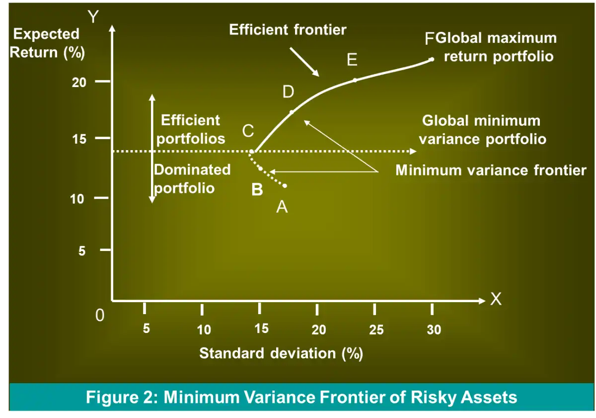
Summarized by Minimum-variance frontier (MVF) of risky assets¹
Lowest possible variance that can be attained for a given portfolio's expected return
Point to the extreme left of the MVF is the global minimum variance portfolio.
The highest point of the MVF represents the global maximum return portfolio.
The line connecting them represents efficient portfolios

Problem Checklist¶

Example 5: Concept of dominance and efficient frontier
- Portfolio A and B are inefficient/dominated.

Efficient Frontier with Margined Short Sales¶

Margined Short sales
- Person sells a second person an asset
- borrowed from a third person (broker)
- Short seller seeks to profit from expected fall in price
- Margin = specified % of market value of the transaction that the short seller deposits with the lender
The point \(\to\) it is possible to construct portfolios that offer the same expected return with a lower variance. Such an efficient frontier dominates the one without margined short sales. (The frontier shifting left…, lower variance for the same returns)

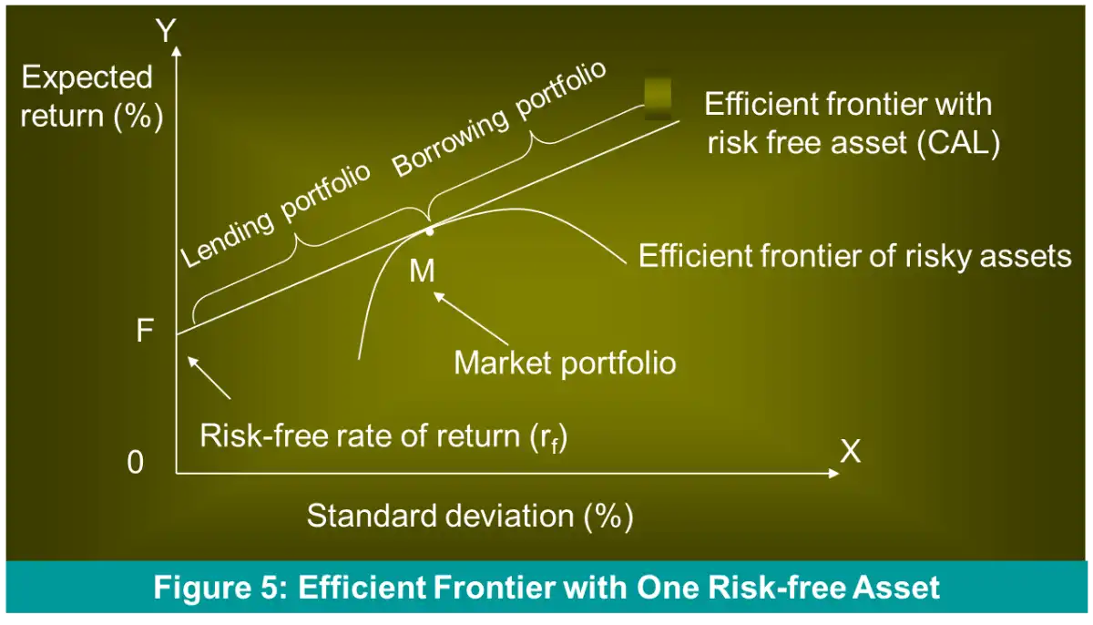
Efficient Frontier with One Risk-free Asset¶

Risk-free security \(\to\) Zero variance denoted by \(\mathbf{F}\)
A risky portfolio \(\mathbf{M}\)
A complete portfolio by combining them \(\mathbf{C}\)
\(w \to\) fraction invested in \(\mathbf{M}\) and remaining (\(1-w\)) \(\to\) \(\mathbf{F}\)

\[ E(r_{c}) = r_{f} + w(E(r_{m}) - r_{f}) \]

\[ \sigma_{c} = w \sigma_{m} \]

\[ E(r_{c}) = r_{f} + \left(\dfrac{\sigma_{c}}{\sigma_{m}}\right)[E(r_{m}) - r_{f}] = r_{f} + \sigma_{c}\left(\dfrac{E(r_{m}) - r_{f}}{\sigma_{m}}\right) \]

Equation of portfolio opportunity set or Portfolio Possible Possibility lines. Termed as the Capital Allocation Line (CAL)
Slope \(= \dfrac{E(r_{c}) - r_{f}}{\sigma_{m}}\)
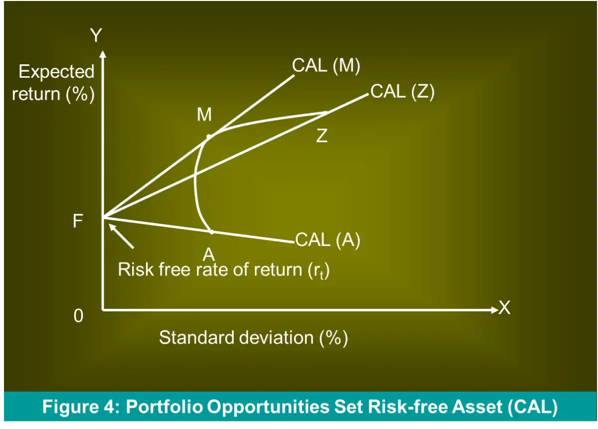
- \(A:\) lower end
- \(Z:\) top end (global maximum returns)
- Highest CAL tangential to point \(M\) on the efficient frontier \(\implies CAL(M)\), offer the best risk-return trade-off.
- Portfolio \(M\) is the best risky portfolio of risky assets.
- Investor can obtain any combination of risk and return on line segment FM. (owned funds)

Efficient frontier with borrowing¶

Extending FM beyond \(M\), opportunities of higher return?
How to exploit these opportunities?
- Borrow funds at risk free rate, \(R_{f}\) and invest the same in risky asset \(M\).
- Known as creating a leveraged, margined or borrowing portfolio
Borrowing \(\implies w_{M} > 1\) and \(w_{R_{f}} < 0\), but \(w_{M} + w_{R_{f}} = 1\)
E.g.
- Investor has 2,00,000
- Borrows 1,00,000 and invests in a risky asset
- Weight of \(M = \dfrac{300000}{200000} = 1.5\)
- Weight of \(R_{f} = 1- 1.5 = -0.5\) \(\implies\) Borrowings are 50% of owned funds.
CAL tangential to efficient frontier of risky assets = new efficient frontier with one risk-free asset, completely dominates the efficient frontier of risky assets

Market Portfolio: \(M\)¶

Add up portfolios of all individual investors, borrowing and lending cancel out
Value of an aggregate risky portfolio is the entire wealth of the economy.
\(\implies\) #doubt Market portfolio is a huge portfolio that includes all traded assets in the same proportion in which they are supplied in equilibrium

CML [Capital Market Line]¶

is a CAL provided by
- Risk-free asset: one-month T-bills
- Risky asset: A market-index portfolio like Down Jones, S&P, NYSE
indicates #doubt
1. locus of all efficient portfolios
2. risk-return relationship
3. appropriate measure of risk for

Investor's Risk Preference¶

Utility score, \(U = E(r) - 0.005A\sigma^2\)
Risk-return indifference curves
Rational investor seeks an efficient portfolio tangent to the highest attainable indifference curve. \(\implies\) Optimal Portfolio

CAPM [Capital Asset Pricing Model]¶

About¶

Explains how asset prices are formed in the market place.
To determine the equilibrium expected return for risky assets
Capital market theories aka asset pricing theories = how prices are determined if investors behaved the way Markowitz's portfolio theory suggests.

Elements¶

CML \(\to\) one-month T-bills + broad index of common stocks
SML (Security Market Line) \(\to\) graphic depiction of CAPM (market price of risk in capital markets)

Capital Market theory says¶

Market compensates or rewards for systematic risk only.
Systematic risk level measured by \(\to\) \(\beta\) coefficient
CAPM links \(\beta \to\) level of required return
Graphic Depiction of CAPM \(\to\) SML

\[ E(r_{i}) = r_{f} + \beta(E(r_{m}) - r_{f}) \]

More familiar

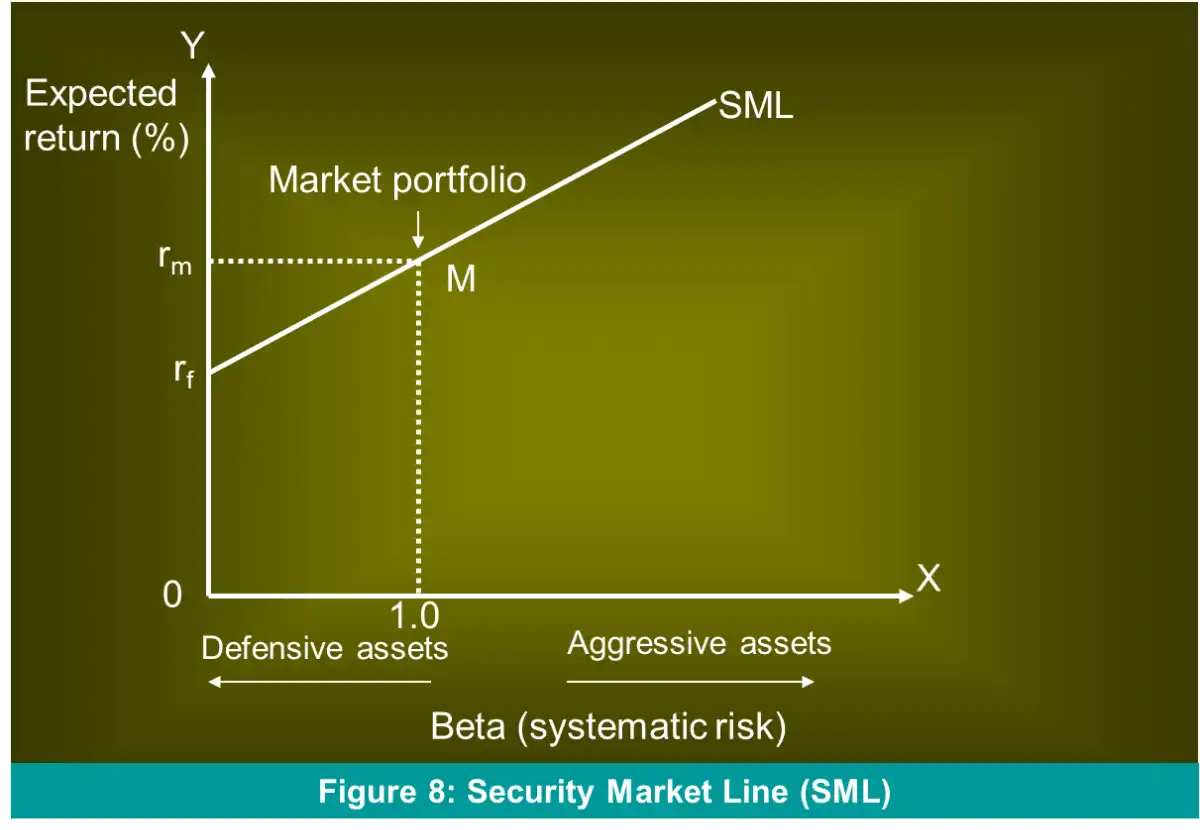
\[ E(r_{i}) - r_{f} = \beta(\underbrace{E(r_{m}) - r_{f}}_{\text{Risk-Premium}}) \]

- Risk-return: Expected return of an individual asset varies directly with its systematic risk \((\beta)\), which measures risk relative to the market portfolio
- T-bills, money market funds, bank deposits \(\to\) Proxy for risk-free rate
- Market Risk-Premium \(= E(r_{m}) - r_{f}\)

Unlevering & Relevering \(\beta\)¶

View all assets of the firm as portfolio (debt + equity)
Market value, \(V\) of firm \(= D + E\)
\(\therefore\) Weighted avg of \(\beta_{D} , \beta_{E} = \beta_{\text{assets}}\)
For an all equity firm, \(\beta_{\text{assets}} = \beta_{E} \leftarrow\) Called Unlevered \(\beta\)
Unlevering: Determination of \(\beta_{\text{assets}}\) from \(\beta_{E}\)
Relevering: Determining \(\beta_{E}\) from \(\beta_{\text{assets}}\) for the proposed financing structure.

\[ \beta_{\text{assets}} = \beta_{\text{portfolio}} = \dfrac{D}{V}\beta_{D} + \dfrac{E}{V}\beta_{E} \]

Extended CAPM¶

CAPM = single factor model (based on \(\beta\))
We can include other factors that affect the security's expected return, too

There are five other major factors that we can talk about.

1. Taxes¶

Investor receives return on security in two forms

Dividend income: which is taxed
Capital gains/losses: of which gains are taxed

In case (either of) these are free-of-tax or taxed at the same rate, the CAPM results hold whether the company pays more or less dividends.

Sample Question

Calculate the Returns from company X and Y after the tax (taxing both dividend yield and capital gain appropriately). And show that the after-tax returns tell a different story about which company has a higher yield.

Modified:

\[ K_{j} = R_{f} + b\beta_{j} + t(D_{j}- R_{f}) \]

where,

\(K_{j}\) required rate of return on security \(j\)
\(R_{f}\) risk-free return
\(b\) relative importance of Beta
\(\beta_{j}\) beta of security \(j\)
\(t\) relative importance of tax effect
\(D_{j}\) dividend yield on security, \(j\)

2. Inflation¶

High inflation \(\implies\) Real return for a security tends to be lower.
If inflation is highly predictable, \(E(R) =\text{Real }K_{f} +\text{Inflation Premium}\)
The higher the covariance of return with unanticipated change in inflation \(\implies\) Lower the expected nominal return
- This covariance is desirable from the investor's standpoint

3. Liquidity¶

Definition

Liquidity refers to the ability to transform a security readily into cash without loss (or at negligible loss, if any)

The bid-ask spread³ of a security may be regarded as a useful measure of its liquidity.
Lower the spread \(\implies\) Higher the liquidity

4. Market Capitalization Size¶

By definition, Market capitalization Size (MCS) is the

\[ \text{MCS} = \text{\# shares O/S} \times \text{Market Price} \]

Higher the MCS, the more secured the investor feels in investing in securities of such a company.

5. Price-Earnings & Market-to-Book Value Ratios¶

Van Horne states

Price/Earnings (P/E) ratio has been observed in realized returns from Securities/equity shares.

Modified CAPM equation with inclusion of P/E ratio

\[ K_{f} = R_{f} +b\beta_{j} - p(\dfrac{P}{Ej} - \dfrac{P}{E_{m}}) \]

where

\(p\) coefficient showing relative importance of a security's \(P/E_{j}\) ratio
\(P/E_{j}\) is the price/earnings ratio of the security \(j\)
\(P/E_{m}\) is the weighted average price/earnings ratio for the market portfolio

Arbitrage Pricing Theory¶

APT is an alternative method of asset pricing.
The APT is based on the concept of arbitrage.
By eliminating arbitrage opportunities, the arbitragers help in developing the state of capital market efficiency in which

All risk-less securities yield the same expected return.

Multifactor Linear Model¶

It relates to the security within a multivariate framework in which the return relationships are linear.
Multivariate framework \(\implies\) Various different factors which influence security returns.
Factors can be classified as
1. Macroeconomic, having pervasive influence
2. Micro (firm-specific) factors

\[ \text{Return} =R_{f} + \beta_{j_{1}} (\bar{r}_{f_{1}}-r_{f}) +\dots+\beta_{jk} (r_{jk}- r_{f}) \]

where

\(k\) is the number of factors that affect an asset (security) returns
\(\bar{r}_{f_{1}},\dots,\bar{r}_{jk}\) are expected returns to factors \(1,\dots,k\)
\(\beta_{j1},\dots,\beta_{jk}\) are sensitivities of an asset (security) to factors 1,…,\(k\)

Investors Risk Management

Risk & Return¶

Problem Checklist¶

Risk & Return of a single asset¶

Sensitivity Analysis¶

Probability (Distribution)¶

Standard Deviation¶

Coefficient of Variation¶

Risk & Return of Portfolio¶

Portfolio Definition¶

Portfolio Expected Return¶

Problem Checklist¶

Portfolio Risk (Two-asset Portfolio)¶

Notable Inferences¶

Problem Checklist¶

Optimal Weights¶

Determination and Correlation¶

Portfolio Selection¶

Process¶

Two broad approaches¶

Efficient Portfolios¶

Problem Checklist¶

Efficient Frontier with Margined Short Sales¶

Efficient Frontier with One Risk-free Asset¶

Efficient frontier with borrowing¶

Market Portfolio: \(M\)¶

CML [Capital Market Line]¶

Investor's Risk Preference¶

CAPM [Capital Asset Pricing Model]¶

About¶

Elements¶

Capital Market theory says¶

Unlevering & Relevering \(\beta\)¶

Extended CAPM¶

1. Taxes¶

2. Inflation¶

3. Liquidity¶

4. Market Capitalization Size¶

5. Price-Earnings & Market-to-Book Value Ratios¶

Arbitrage Pricing Theory¶

Multifactor Linear Model¶

Other Topics¶

Brealey¶

PC¶