Options
Definition
An option gives the holder the right, but not the obligation to buy or sell a given quantity of an asset on (or before1) a given date at prices agreed upon today.
Terminology
| TERM | DETAILS | ||
|---|---|---|---|
| Index Options | Underlying = Index. European/American | ||
| American Options | can be excised at any date, up to expiration. (Most traded) | ||
| European Options | only at the expiration date. (Easier to analyze) | ||
| Exercising the option | The act of buying or selling the underlying asset. | ||
| Stock options | Underlying = individual stocks | Holder the right to buy/sell shares at the specified prices. | |
| Buyer | Paying the option premium | Has the right to exercise his option. | |
| Writer/Seller | Receives the option premium | Obliged to sell/buy if buyer exercises. | |
| Call Option | Holder has right (not obligation) | to buy asset by a certain date for a certain price. | |
| Put Option | […] | to sell […] | |
| Option Price/Premium | Price option buyer pays the seller | ||
| Expiration Date | Date specified in the options contract | a.k.a. exercise date or strike date | |
| Strike Price | Price specified in the options contract | a.k.a. exercise price | |
| In-the-Money (ITM) Option | that would lead to a positive cashflow to the holder if exercised immediately | Call opt on the index if spot price \(\gt\) strike price. (Much higher: deep ITM) | |
| Put opt on the index if strike price \(\gt\) spot price (sell at a higher price than market) | |||
| At-the-Money (ATM) Option | […] zero cashflow […] | […] spot price \(=\) strike price. | |
| Out-of-the-Money (OTM) Option | […] negative cashflow […] |
[…] spot price \(\lt\) strike price. |
|
| Option Premium = | Intrinsic value + time value |
||
| Intrinsic Value of an Option | Intrinsic value = ITM else 0 (if call is OTM). | \(\max(0,S_{t}-K)\) for call. | |
| Time Value of an Option | = Premium - Intrinsic value. The longer the time to expiration, the greater the time value | Maximum time value option is ATM. At expiration, no time value. |
Characteristics of Options Payoffs
Payoff for derivative contracts = likely profit/loss due to change in price of underlying asset.
For options, the optionality characteristics creates:
- Non-linear pay-off implies
- losses for the buyer are limited, but profits are potentially unlimited.
- profits for the seller are limited, but losses are potentially unlimited.
- Option Premium
Call Option
Buyer has right to buy the underlying asset at strike price
- You "call in" an asset, when exercising a call option.
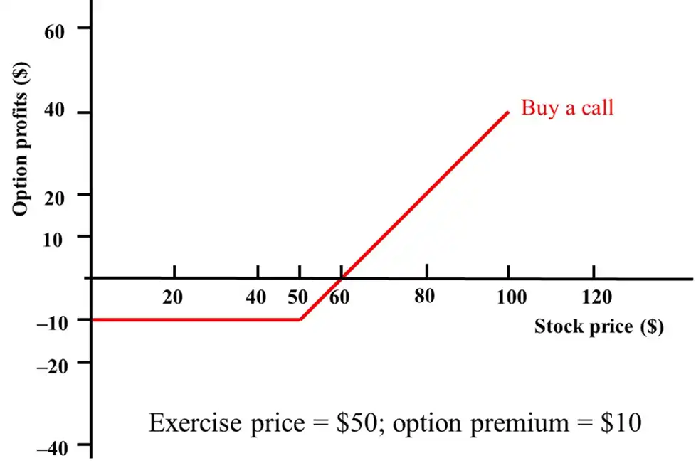
Long Call (Buyer)
- Higher the \(S_{t}\), more the profit he (buyer) makes.
- If \(S_{T} \lt\text{Strike}\) , he leaves the option unexercised. The buyer loses the premium he paid.
Interpretation
To identify the strike price of a call, see where the elbow breaks
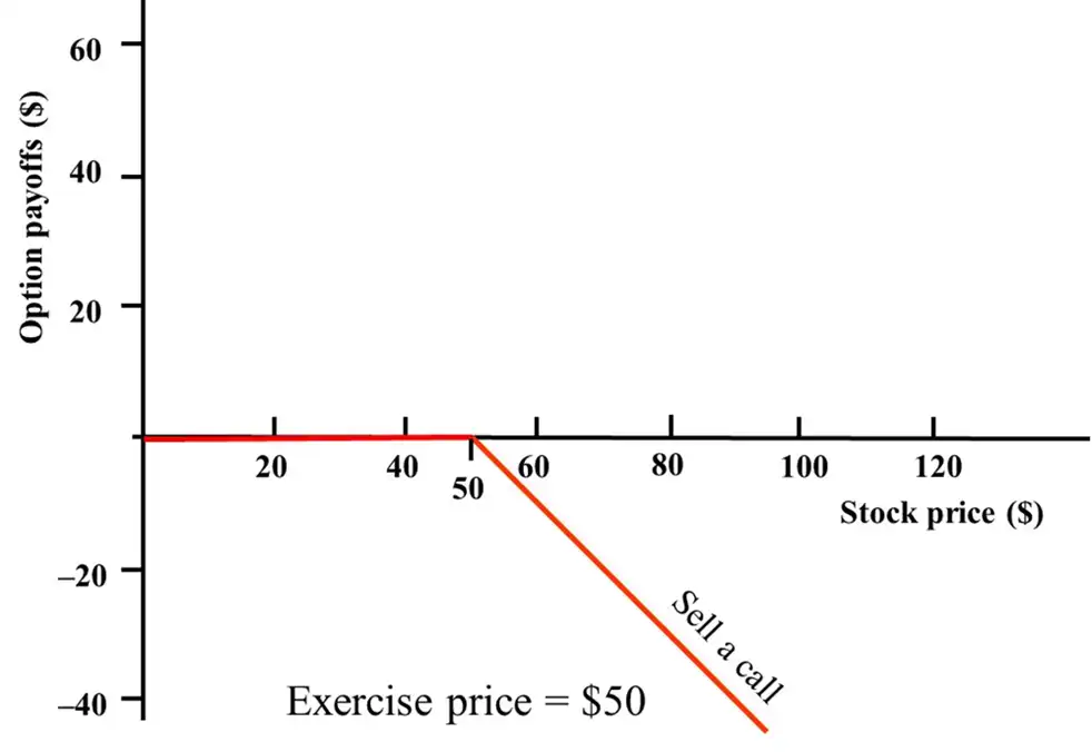
Short Call (Writer)
- Higher the \(S_{t}\), more the loss he (writer) makes.
- If \(S_{T}\lt Strike\), option left unexercised. The writer keeps the premium (profit)
Pricing at Expiration
- American = European (with same characteristics) at expiration
- If the call is ITM, price = \(S_{T}-K\)
- Out of the money, worthless, price = \(\max(S_{T}-K,0)\)
Put Option
Buyer has the right to sell the underlying asset at strike price
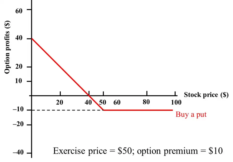
Long Put (Buyer)
- Lower the \(S_{t}\), more the profit he makes. (He can sell at a higher price and buy again at a lower price)
- If \(S_{T} \gt\text{Strike}\), option left unexercised. Buyer loses the premium he paid to buy the put option.
Short Put (Writer)
- Lower the \(S_{t}\), more the loss he (writer) makes. (Buyer's profit is the seller's loss)
- If \(S_{T}\lt Strike\), option left unexercised. The writer keeps the premium (profit)

Pricing at Expiration
- In the money: \(E - S_{T}\)
Option Value
Definition
Speculative Value = \(\text{Option Premium}-\text{Intrinsic Value}\)
And thus,
Option Quotes
- Remember that if your \(\text{Strike}\gt\text{Current Price}\), you will wish to sell it (for more, at strike) \(\implies\) Put option is ITM \(\implies\) Call option is OTM
| Recent Price (IBM) |
Option/Strike | Exp. | Call Vol. |
Call Last |
Put Vol. |
Put Last |
| 167.3 | 162.5 | Jul | 21 | 5.85 | 145 | .89 |
| 167.3 | 165 | Jul | 108 | 3.95 | 150 | 1.48 |
| 167.3 | 170 | Jul | 212 | 1.25 | 335 | 3.95 |
| 167.3 | 170 | Aug | 1449 | 3.15 | 1518 | 6.75 |
| 167.3 | 170 | Sep | 156 | 3.91 | 264 | 7.71 |
| 167.3 | 175 | Sep | 101 | 2.18 | 78 | 11.05 |
- \(170 \gt 167.3\) \(\implies\) Put option is ITM, Call is OTM
- 212 call options with this exercise price were traded
- The Call option itself traded for $1.25 i.e. \(C = 1.25\)
- The option is for 100 stocks
- So, cost of buying this call = $125 (+ commissions, if any)
- 335 put options with this exercise price were traded
- \(P = 3.95\)
- 100 shares of stocks, so cost = 395 (+ commissions)
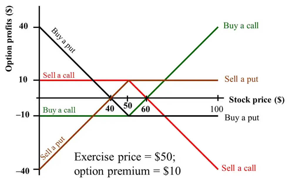
Combinations of Options
- Use puts and calls as building blocks to make more complex option contracts.
Protective Put Strategy
Optimistic: Downside protection and upside potential.
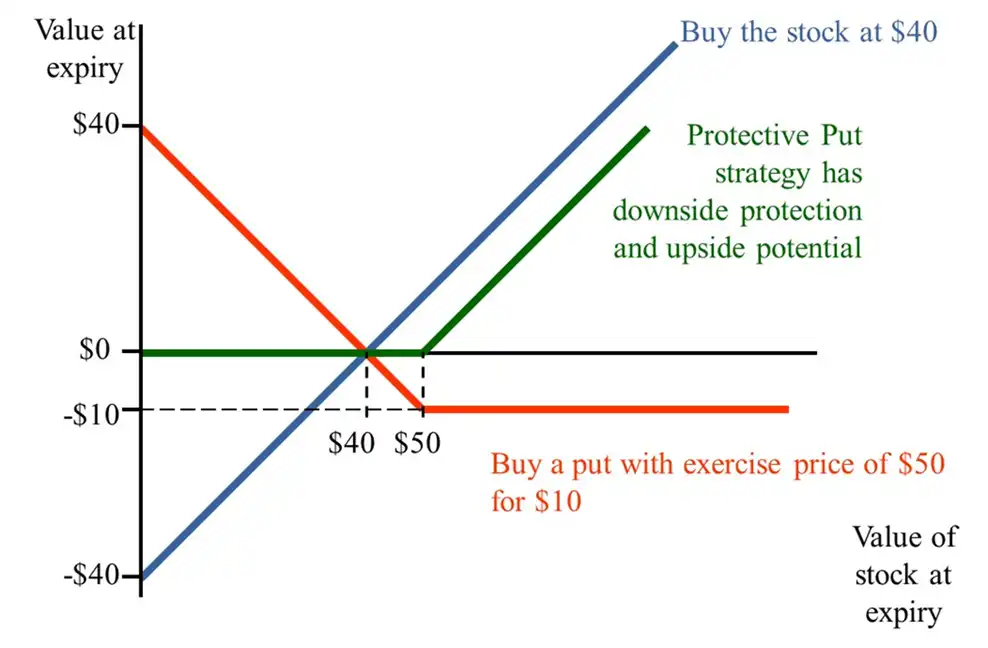
- It sees a profit, because option premium = 10, strike price = 50 and \(S_{0}\) = 40
- Alternate scenario, if Strike price was 45, then draw the same diagram and you will see that the green line (of the Protective Put strategy) starts from -5 and elbows at 45 then goes up, touching the x-axis at 50
Covered Call Strategy

- Since the loss potential in selling a call is infinite, we can "cover the call" by buying the same stock.
Put-Call Parity
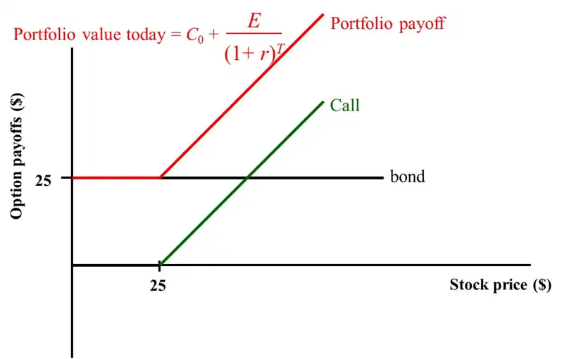
This is a portfolio with
- Call with strike \(K = 25\)
- Bond with future value \(25\) (same as \(K\))
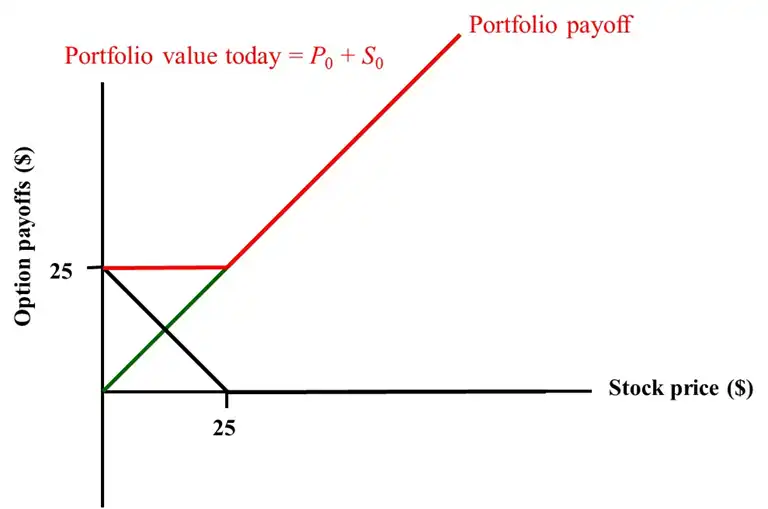
Portfolio with
- Share of stock with price \(S_{0} = 25\)
- Put with a strike \(K = 25\)
They have the same value!
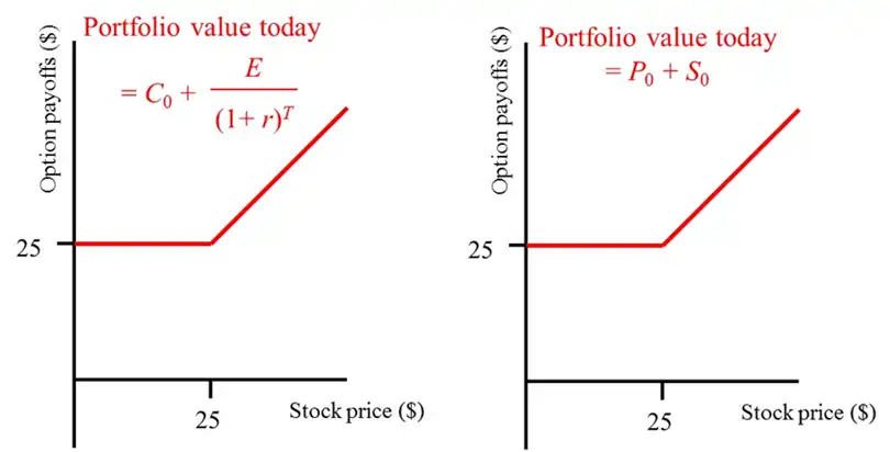
Thus they have the same value today:
Or in words
Holds when Put and Call have the same
- Exercise price, \(C=P\)
- Expiration Date, \(T\)
Hence, we can replicate buying a stock by buying a call, selling a put2 and buying a zero coupon bond.
- We can also find the price/value of a put if we know the price of a call option, duration and strike price.
Valuing Options (before expiration)
American Call
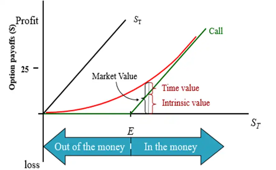
- Market value is the vertical distance between the Red curve and horizontal axis.
- Time value is the vertical distance between Red curve and green call value line.
- Intrinsic value is the vertical distance between the green call value line and horizontal axis.
Thus, market value lies between \(S_{T}\) curve and the Intrinsic call value line.
Option Value Determinants
| Determinant | Call | Put |
|---|---|---|
| \(S_{0}\), current price | + | - |
| \(K\), strike | - | + |
| \(r\), risk-free interest rate | + | - |
| \(\sigma\), volatility in stock price | + | + |
| \(T\), expiration | + | + |
| Dividend paying | - | + |
Mental Model
Think of value as "value to the holder/buyer"
- More the stock price,
- the buyer of call, will buy asset at the strike \(\implies\) profits for him.
- the buyer of put, will have to pay a higher price. Sad for him
- More the strike,
- higher the price buyer of call, needs to pay. Sad for him
- the buyer of put, will get a higher strike. profits for him
- If \(r\) is high,
- call buyer has to borrow "less money" to pay the strike price.
- put buyer will discount the strike price, and feel scammed.
- If there is higher volatility in stock price, the buyer has the kill-switch, it is always a risk for the seller. Good for buyer
- More time to expiration, means more time to act. Who has the kill-switch? The buyer. So higher risk for the seller. Good for buyer
Additional Points for American Options
This should ALWAYS hold!
- \(C_{0} \lt S_{0}\) (no arbitrages)
- \(\max(S_{0}-K,0) \lt C_{0}\) (meaning, strike should be higher than \(S_{0}\), no arbitrages)
- \(S_{0} = 0 \implies C_{0} = 0\)
- \(S_{T} \gg K \implies C_{0} \to S_{0} - \dfrac{K}{(1+r)^T}\)
Option Pricing Formula
Binomial Option Pricing Model
- \(S_{0}= \$25\)
- At \(t=1\), \(S_{1}\) is either 15% more or 15% less (28.75 or 21.25)
- What is the value of at-the-money option?
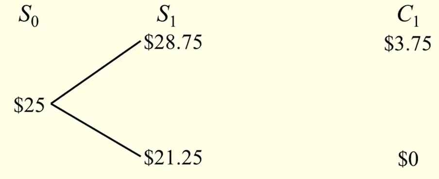
- The payoffs in the next period are indicated as \(C_{1}\)
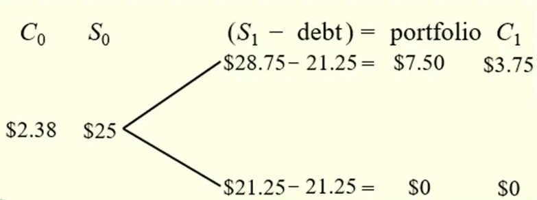
- Replicate the payoffs of call option with a levered position in the stock
- Borrow the PV(21.25, lower point) and buy one stock
- Thus, net payoff is now 7.5 or 0
- \(25 - \dfrac{21.25}{(1+R_{f})}\)
Thus, value the call option today as half the value of levered-equity portfolio (the expected value of the portfolio.)
Delta
- Delta of a call option is positive,
- Delta of a put option is negative
Thus, we can find amount borrowed as
The Risk-Neutral Approach
- Value of option, \(V(0)\) → the value of the replicating portfolio
- Equivalent method = risk-neutral valuation
- \(q\) is the risk neutral probability for an "up" move (\(U\))
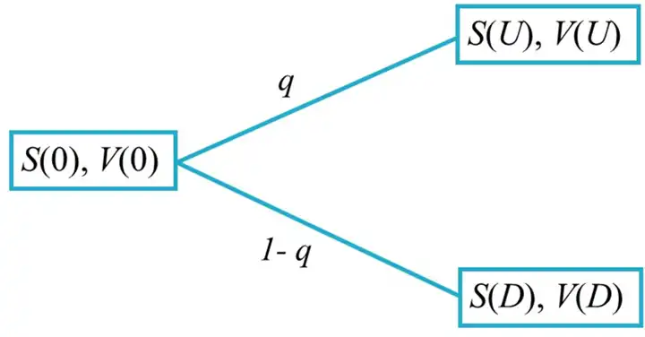
- \(S(U)\) and \(S(D)\) are asset prices ("up" and "down" moves)
- \(V(U)\) and \(V(D)\) are option values ("up" and "down" moves)
Thus we can find \(q\) since we already observe \(S(0)\), and have speculations about what "up" and "down" movements will show up at which \(R_{f}\) rate of interest.
And then \(C(U)\) and \(C(D)\) can be derived since we known \(K\).
Black-Scholes Option Pricing Model
Geometric Brownian Motion
A simple and well-known equation that models the way in which stock prices fluctuate.
\(\implies\) The stock returns will have lognormal distribution \(\implies\) Log of stock returns will follow normal distribution.
Assumptions of Black-Scholes-Merton Model
- Underlying asset
- Price follows Geometric Brownian Motion (\(\log\text{-}N\))
- Constant \(\sigma\)
- No Dividends
- Market
- Constant \(r_{f}\)
- Perfect liquidity and continuous trading
- No transaction costs or taxes
- No limits on shortselling
- No arbitrage
- Options
- European style options
Black-Scholes formula for prices of European calls and puts on a non-dividend paying stock:
Correction: In the K&J source, the formula for the \(P\) have the \(d_{1}\) and \(d_{2}\) the other way, which is wrong. The formula above, given here are correct.
where,
- \(d_{1} = \dfrac{\ln \dfrac{S}{X}+\left(r+\dfrac{\sigma^{2}}{2}\right)T}{\sigma \sqrt{ T }}\)
- \(d_{2} = d_{1}-\sigma \sqrt{ T }\)
- Continuously compounded, \(r = \ln(1+\bar{r})\) where \(\bar{r}\) is interest rate per annum
- \(N()\) is the cumulative normal distribution.
- \(N(d_{1})\) is the delta of the option (= measure of change in option price with respect to the change in price of underlying)
- \(\sigma\) = measure of volatility = annualized standard deviation
- \(\sigma = \sigma_{\text{annual}} = \sigma_{\text{daily}} \times \sqrt{ \text{\# of trading days per year} }\)
- On average, 250 trading days per year.
- \(X\) is the exercise price
- \(S\) is the spot price
- \(T\) is time-to-expiration (in years)
Consistent Notation
I would prefer writing it with more familiar notation:
where,
- \(d_{1} = \dfrac{\ln \dfrac{S_{0}}{F_{0}}+(r + \dfrac{\sigma^2}{2})T}{\sigma_{\text{annual}}\sqrt{ T }}\)
- \(d_{1}-d_{2}=\sigma_{\text{annual}}\sqrt{ T }\) \(\implies\) \(d_{2} = d_{1}-\sigma_{\text{annual}}\sqrt{ T }\)
Pricing Index Options
Assumption of Black-Scholes Options Pricing Model
Investors can purchase, without cost, the underlying stocks in the exact amount necessary to replicate the index.
- Stocks are infinitely divisible
- Index follows a diffusion process \(\ni\) continuously compounded returns of index follow Normal distribution
Hence, index options should be valued in the same way as ordinary options on common stock.