Lecture 29 Cumulative Prospect Theory II

• Non-linear preferences (contd.)
  • Principle of diminishing sensitivity: impact of given change in probability diminishes with its distance from the boundary
  • Evaluation of outcomes - Boundary to distinguish losses and profits = reference point
  • Evaluation of uncertainty - two natural boundaries (corresponding to certainty scale)
    • certainty
    • impossibility
  • E.g. \(0.9 \to 1.0\) or \(0 \to 0.1\) has more impact than \(0.3 \to 0.4\) or \(0.6 \to 0.7\)
    • \(\implies\) Diminishing sensitivity, concave near 0 and convex near 1 "\(\sim\) shaped"
  • For uncertain prospects:
    • subadditivity for very unlikely
    • super-additivity for near certainty
    • very small probabilities are either greatly overweighted or neglected altogether

• Scaling

  • K&T suggested $$v(x) = \begin{cases} x^\alpha \ & \text{if } x \geq 0 \ -\lambda(-x)^\beta & \text{if } x \lt 0 \end{cases} $$
  • \(\alpha:\) coefficient of diminishing marginal sensitivity to gains
  • \(\beta:\) coefficient of diminishing marginal sensitivity to losses
  • We are referring these two as exponents
  • \(\lambda:\) coefficient of loss-aversion
  • Functional forms of weighting function
  • \[ w^+(p) = \dfrac{p^\gamma}{(p^\gamma + (1-p)^\gamma)^{1/\gamma}} \]
  • \[ w^-(p) = \dfrac{p^\delta}{(p^\delta + (1-p)^\delta)^{1/\delta}} \]
    • \(\gamma\) and \(\delta\) determine the curvature function, different for losses and gains.
  • When a non-linear regression procedure was used to estimate parameters:
    • The median exponents (\(\alpha = \beta\) ) \(=0.88\)
    • The median \(\lambda = 2.25\) indicating loss aversion
    • For the weighting function, \(\gamma = 0.61\) and \(\delta = 0.69\)
  • 
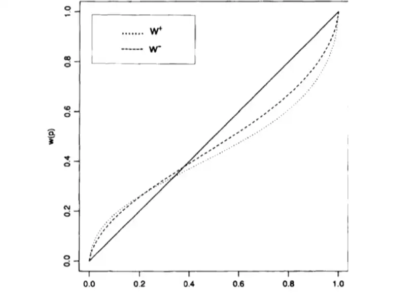
    • concave and steep at low
      • overweight for very small probabilities
    • convex after: shallow in the middle range steep at high
      • underweight moderate and high probabilities
    • CE > EV: risk seeking
    • CE < EV: risk aversion
    • CE = EV: risk neutral
  • Empirical evidence
  • CE: average amount the subjects were ready to pay (say $78) to obtain an EV of $95 so risk averse.
  • Gain, high \(p \to\) Averse
  • Loss, high \(p \to\) Seeking
  • Gain, medium \(p \to\) Averse
  • Loss, medium \(p \to\) Seeking
  • Gain, low \(p \to\) Seeking
  • Loss, low \(p \to\) Averse
  • Improvements offered by CPT

  Specification of choice under uncertainty	EUT	CPT
  Objects of choice	Probability distribution over wealth	Prospects framed in terms of gains and losses
  Valuation rule	\(E[U]\)	\(V(f) = V(f^+) + V(f^-)\)
  Characteristic of the map \(: \text{Uncertain Event} \to \text{Subjective}\)	\(U \sim\) convex function of wealth	Value function: s-shaped Weighting function: inverse s-shaped

  • Curvature of weighting function: reflection pattern of attitude to risky prospects
  • Overweighting of small probabilities: lottery and insurance
  • Underweighting of high probabilities: risk aversion in choice between probable gains vs sure win.
  • Curvature of value function: risk-aversion of gains, risk seeking for losses
  • Asymmetry of value function: loss aversion, extreme reluctance to accept mixed prospects
  • Shape of weighting function: certainty effect
  • The Value function
  • \(r \neq 0\) (if \(r=0\), its the original K&T value function)
    • \[v(x) = \begin{cases} (x-r)^\alpha & \text{if } x\geq r \\ -\lambda(r-x)^\beta & \text{if } x \lt r \\ \end{cases}\]
  • Application - Asian Disease Problem 1 ^83c303
  • Asian disease expected to kill 600 people
  • Two alternative programs to combat the disease
    • \(A:\) (200) people will be saved (for sure)
    • \(B:\) \((600, \dfrac{1}{3})\) else no one
  • Choices: \(A \to 72\%\) and \(B \to 28\%\)
  • \(A\) can be written as \((200,1;400,0)\)
  • \(B\) can be written as \((600, \dfrac{1}{3}; 0 \dfrac{2}{3})\)
  • Application - Asian Disease Problem 2 ^6cbd95
  • Same context
  • Two alternatives
    • \(C:\) (400) people will die (for sure)
    • \(D:\) \((0, \dfrac{1}{3})\) else 600 die.
  • Choices: \(C \to 22\%\) and \(D \to 78\%\)
  • \(C: (400)\) and \(D: (600, \dfrac{2}{3})\)
  • Application Questions
  • Few effects
    • Framing (reference point changed)
    • Certainty
    • Reflection (gains and losses are reflections)
    • loss aversions
    • preference reversal
  • Calculate the value functions using functional forms and estimated parameters and check its efficacy
  • Problem 1 states "how many lives saved"? \(r=0\)
  • Problem 2 states "how many die"? \(r = 600\)
  • Value Functions - Problem 1
  • \(V(A) = v(200) = 200^{0.88} \cong 105.90\) for \(w^+(1)= 1\)
  • \(V(B) = w^+\left( \frac{2}{3} \right)v(0) + w^+(\frac{1}{3})v(600) \cong 67.24\)
  • \(V(A) = 105.90 \gt V(B) = 67.24\) and so \(A \succ B\)
  • Value Functions - Problem 2
  • We see that
  • \(V(D) = -165.43 \gt V(C) = -238.28\) and so \(D \succ C\)