Lecture 28 Cumulative Prospect Theory I
- Stochastic Dominance
- \(A = (x_{1},p_{1};\dots,x_{n},p_{n})\)
- \(B = (y_{1},p_{1};\dots;y_{n},p_{n})\)
- \(B\) weakly stochastically dominates \(A\) if \(x_{i} \leq y_{i}\) for all \(i\)
- strictly if the above definition PLUS \(x_{i} \lt y_{i}\) for some \(i\)
- An example of 4 gambles
- B dominates A but C was preferred to D
- Though \(C \sim A\) and \(D \sim B\)
- Due to ambiguity in presentation
- But when \(G\) is introduced, people started to \(A \succ G \succ B\) \(\implies\) \(A \succ B\)
- PT fails to explain this: "Why are dominated prospects eliminated in the editing phase?"
-
Cumulative Prospect Theory (CPT)
- incorporates the cumulative functional
- extends theory to uncertain and risky prospects (w/ any number of outcomes)
- unified treatment of risk and uncertainty
- Address five major phenomena of choice
-
Framing effect ^89062f
- Rational theory of choice assumes Description invariance
- But there are variations due to framing options
- Non-linear preferences ^1cf13b
- Utility of a risky prospect is linear in outcome probabilities
- Allais's famous example: probability difference 0.99 and 1.00 has more impact on preferences than 0.10 and 0.11.
- \(\implies\) Non-linear preferences
- Major difference between PT & CPT: allowance for different weights for gains and losses
- Source Dependence - Ellsberg Paradox^9b4bb6
- Willingness to be on an uncertain outcome depends on
- degree of uncertainty
- source of uncertainty
- Ellsberg observed that people prefer betting on an urn contain equal number of red and green balls rather than unknown proportions
- More recent evidence: people are willing to bet on event in their area of competence than on a matched chance event (where they have uncertainty)1
- Ambiguity Aversion
- Urn 1 and 2
- Gamble A: unknown proportion
- Gamble B: 50-50
- Preference is inconsistent, with EUT
- People generally choose the urn where they are more certain about the outcome, even if it contrasts their prior beliefs.
- Willingness to be on an uncertain outcome depends on
- Risk Seeking ^58969d
- These choices are consistently observed in:
- People prefer a small probability of winning a large price \(\gt\) expected value of that prospect
- Choosing between a sure loss \(\lt\) substantial probability of a larger loss
- These choices are consistently observed in:
- Loss aversion ^8dfee5
- Losses loom larger than gains in case of risk and uncertainty
- Slope of utility function is more steeper in the domain of losses than that of gains.
- The New Decision Weights Function
- Solved by rank-dependent or cumulative functional proposed by Quiggin (decision under risk) and Schmeidler (decision under uncertainty3)
- Revised model transforms the entire cumulative distribution function
- Applies cumulative functional2 to losses and gains separately
- Setup
- \(S:\) set of events. Each state \(s \in S\) has the consequence \(x \in X\)
- Uncertain prospect \(f\), sequence of pairs \(f(s) = f(x_{i},A_{i})\)
- \(x_{i}\) yields if \(A_{i}\) occurs
- Outcomes are Sorted in increasing order \(x_{i} \gt x_{j} \iff\) \(i \gt j\)
- \(A_{i}\) is a partition of \(S\)4
- If \(f(s)\) is given by a probability \(\implies\) "risky" prospect
- \(p(A_{i})= p_{i}\)
- \((x_{i},p_{i})\)
- Value function has two components
- \(V(f) = V(f^+)+V(f^-)\)
- \(f^+\) and \(f^-\) are positive and negative parts of the prospects
- \(f^+(s) = f(s)\) if \(f(s) \gt 0\) else \(f^+(s) = 0\)
- \(f^-(s) = f(s)\) if \(f(s) \lt 0\) else \(f^-(s) = 0\)
- \(V(f) = V(f^+)+V(f^-)\)
- For a mixed or regular prospect (\(* = +/-\))
- \(V(f^*) = \sum_{i=0}^n \pi_{i}^* v(x_{i})\)
- Decision weights:
- For \(0,1,2\dots i\dots n-1\)
- \(\pi_{i}^+ = w^+(p_{i}+\dots+p_{n})- w^+(p_{i+1}+\dots+p_{n})\)
- For \(1-m\dots,i,\dots-3,-2, -1, 0\)
- \(\pi_{i}^- = w^-(p_{-m}+\dots+ p_{i})- w^-(p_{-m}+\dots+p_{i-1})\)
- And
- \(\pi_{n}^+ = w^+(p_{n})\) and
- \(\pi_{-m}^- = w^- (p_{-m})\)
- \(w^+\) and \(w^-\) are strictly increasing functions which are \(w^*(0)=0\) and \(w^*(1) = 1\)
- Example
- Win even \(x\) or lose odd \(x\)
- consequences of \(f\) = \((-5,-3,-1, 2,4, 6)\)
- So, \(f^+ = \left(0, \dfrac{1}{2}; 2, \dfrac{1}{6}; 4, \dfrac{1}{6}; 6, \dfrac{1}{6}\right)\)
- and, \(f^+ = \left(-5, \dfrac{1}{6}; -3, \dfrac{1}{6}; -1, \dfrac{1}{6}; 0, \dfrac{1}{2}\right)\)
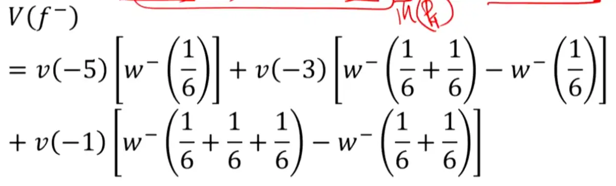
- Then evaluate the entire value function by adding the two components \(V(f) = V(f^+) + V(f^-)\)
-
Even though the former probability is vague. ↩
-
A functional is just a function that takes in a function as an argument (e.g. a curve, is represented by \(f(x) = 2x^2+4\)) and returns a single number as result (e.g. the arc length) ↩
-
A #doubt what is the difference between risk and uncertainty
- I think "uncertain" means, we don't know the probabilities
- When probabilities are known, it is referred to as "risky" ↩ -
Partitions are mutually exclusive and their unions form \(S\) ↩