Lecture 25 Prospect Theory Evaluation

Sairam

PT - Evaluation
- Once editing phase is done, evaluate each of the edited prospects, and choose the prospect with the highest value.
- $V:$ Value function (overall value of edited prospect)
- expressed in terms of two scales
  - $v(x):$ assigns subjective value to each outcome $x$. Deviations from the reference point (gains/losses)
  - $\pi(p):$ impact of probability $p$ on overall value of prospect. Decision weight.¹
- $(x,p;y,q)$
  - $\implies$ $(x,p;y,q;0,1-p-q)$.
  - Prospect is strictly positive if $x,y \gt 0$ and $p+q = 1$ (i.e. all outcomes are positive) and strictly negative if all outcomes are negative.
  - regular if neither strictly positive nor strictly negative
  - Corner example: $(400,0.4; 200, 0.5)$²
- If $(x,p;y,q)$ is regular
  - $V(x,p;y,q)$ = $\pi(p)v(x) + \pi(q)v(y)$
  - where $v(0)=0,\ \pi(0)= 0,\ \pi(1) = 1$
- $V$ defined on prospects. $v$ defined on outcomes
  - $V(x,1.0) = V(x) = v(x)$ for sure/certain prospects
  - Generalization of $EUT$ by relaxing expectation principle
- Situation (coin toss) for a regular prospect
  - Heads: gain $20
  - Tails: lose $10
  - $V(20,0.5;-10,0.5)=$ $\pi(0.5)v(20) + \pi(0.5)v(-10)$
- Rules for strictly positive/negative prospects
  1. Riskless Component (min gain/loss which is certain to be obtained)
  2. Risky Component (additional gain/loss which is actually at stake)
  3. Evaluation: If $p+q = 1$ and $x \gt y \gt 0$ or $x \lt y \lt 0$³
    - $\implies$ $V(x,p;y,q) =$ $v(y) + \pi(p)[v(x) - v(y)]$
    - $=$ riskless component + value-difference between outcomes $\times$ weight associated with more extreme outcome (here $x$)
    - Essential feature: decision weight is applied to the risky component $v(x) - v(y)$ and not the riskless component $v(y)$
- Markowitz #economist was the first one to propose, "Utility should be defined to gains and losses rather than on final asset positions..."
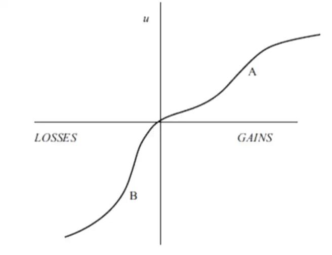
  - Proposed utility function which has concave and convex regions in both +ve and -ve domains
- Many attempts were made to replace probabilities with more general weights. So that we have a perception of risk rather than the outcome's probability directly. To explain aversion for ambiguity.⁴
- Effects of reference point are accounted for by assuming that values are attached to changes rather than final states. (hence a different rule for strictly positive/negative prospects )
- Anomalies of preferences implied by PT are expected to occur and can be used by the decision-maker, who cannot rely on expected utility theory henceforth.

NOTE: $\pi$ is not a probability measure ↩
is not strictly positive because the probabilities don't add up to $1$ meaning, there is a zero outcome possible. Making it not strictly positive. ↩
Strictly positive: $y$ is smaller... so $v(x) - v(y) \gt 0$. Strictly negative: again, y is the smaller loss. The one that is closer to zero is the smaller loss or gain. ↩
In expectation theory, we directly do a sumproduct of outcome values and their probabilities. (Rationally good) but in Prospect theory we do a sumproduct of perceived value (subjective) and decision weight of the probability. ↩