Solow's Model

Production Function (Intensive Form)

• Given production function \(Y=F(K,L)=K^{\alpha}L^{1-\alpha}\) (\(K,L\) are inputs) where \(0<\alpha<1\) is constant lying between 0 and 1.
• Production Function in intensive form: (Output per worker)
• Output per worker: \(y = \dfrac{Y}{L} = \dfrac{K^{\alpha}L^{1-\alpha}}{L} = (\dfrac{K}{L})^{\alpha} = k^{\alpha}.\)
• \(k\) is Capital per worker. \(y=k^{\alpha}\).

• We also assume that

  1. If \(k\) is zero, \(y = (0)^{\alpha} = 0\), so the Production function is Passing through origin.
  2. The first derivative is \(\dfrac{dy}{dk} = \alpha \cdot k^{\alpha-1} > 0\) (increasing function).
  3. The second derivative is \(\dfrac{d^{2}y}{dk^{2}} = \alpha(\alpha-1)k^{\alpha-2} < 0\).

• Since the second derivative is negative, the graph would be Concave.

• If \(K \uparrow \rightarrow \frac{K}{L} \uparrow \rightarrow k \uparrow \rightarrow y \uparrow\): with more capital per worker, firms produce more output Per worker.
• However, there are diminishing returns to Capital per worker.

Derive Capital Accumulation equation

\[\dot{K} = sY - \delta K\]

where,

• \(\dot{K}\) is instantaneous change in \(K\), \(\dot{K} = (K_{t+1}-K_{t})\).
• \(\dot{K}\) is net investment.

If we wish to find the growth rate in capital

\[\dfrac{\dot{K}}{K} = \text{growth rate in capital} = \dfrac{K_{t+1}-K_{t}}{K_{t}}\]

Now, in a closed economy whatever is saved is invested.

\[ Y = C + I + G \]

And so,

\[ \underbrace{Y-C-G}_{\text{Gross Savings}} = \underbrace{Y-C-T}_{\text{Private Savings}}\quad + \underbrace{T-G}_{\text{Public savings}} = \underbrace{I}_{\text{Gross investment}} \]

Gross Savings \(S = sY = I\) (Gross Investment), where \(s\) is the Saving Propensity or Savings ratio and It is given exogenously.

So, from capital accumulation equation:

\[\boxed{\dot{K} = sY - \delta K}\]

Meaning,

\[ \text{Net Investment} = \text{Gross Savings} - \text{Depreciation} \]

Here, \(\delta\) is depreciation rate and \(\delta K\) is the total depreciation of capital stock. That occurs during Production.

Capital Stock Change

Conditions

• So, \(\dot{K} = sY - \delta K\).
• \(\dot{K} > 0\): Capital stock is increasing. This happens if Gross investment (\(sY\)) is greater than depreciation (\(\delta K\)).
• If \(sY > \delta K\), then \(\dot{K} > 0\) (Replace the existing capital and also have surplus investment. Invest 10 machines while we needed to replace only 5.)
• If \(sY < \delta K\), then \(\dot{K} < 0\) (The capital in the economy is going to fall since we invested less than what was required)
• If \(sY = \delta K\), then \(\dot{K} = 0\), capital stock unchanged.

Interpretation

• The number of machines added in the economy (\(sY\)) compared to the number of machines which needed to be added to the economy to keep the Capital unchanged (\(\delta K\)).
• If we are adding more machines than what is needed to be added to keep the capital unchanged, definitely capital will increase.
• If we are adding less machines than what is needed to keep the capital unchanged then, capital is going to fall.

Capital Accumulation in Per Capita Form (Solow's Equation Derivation)

Now, let's Convert the capital accumulation equation into per capita form.

Key equation of Solow Model (from #Derive Capital Accumulation equation)

\[\dot{K} = sY - \delta K\]

We know that \(k = \dfrac{K}{L}\) \(\implies\) \(\ln k = \ln K - \ln L\).

Taking time derivatives on both sides by differentiating w.r.t to time:

\[ \dfrac{d\ln k}{dt} = \dfrac{d \ln K}{dt} - \dfrac{d \ln L}{dt} \]

which gives

\[ \dfrac{1}{k}\dfrac{dk}{dt} = \dfrac{1}{K}\dfrac{dK}{dt} - \dfrac{1}{L}\dfrac{d L}{dt} \]

and can be written as

\[\frac{\dot{k}}{k} = \frac{\dot{K}}{K} - \frac{\dot{L}}{L}\]

Assumption

Assumption is that labor force is exogenously growing at the rate (\(n = \dfrac{\dot{L}}{L}\)).

• This is one of the weaknesses of this model
• The model failed to distinguish Population growth rate and Labor growth rate.

---

\[\frac{\dot{k}}{k} = \frac{\dot{K}}{K} - n\]

Substitute \(\dot{K} = sY - \delta K\):

\[\frac{\dot{k}}{k} = \frac{sY - \delta K}{K} - n.\]

Dividing by \(L\) in the numerator and denominator like so, \(\dfrac{sY/L}{K/L}\) to get their intensive form.

\[\frac{\dot{k}}{k} = \frac{sy}{k} - (\delta+n)\]

Multiply by \(k\):

\[\dot{k} = sy - (n+\delta)k\]

Since \(y = k^{\alpha}\),

\[\boxed{\dot{k} = s k^{\alpha} - (n+\delta)k}\to \text{(Key equation of Solow model)}\]

Two expressions derived

• \(\dot{K} = sY - \delta K\)
  • \(\dot{K}\): net investment,
  • \(sY\): gross investment,
  • \(\delta K\): replacement cost
• \(\dot{k} = s k^{\alpha} - (n+\delta)k\)
  • \(\dot{k}\): net investment per worker,
  • \(s y\): gross investment per worker,
  • \((n+\delta)k\): replacement cost per worker.

---

• The term '\(nk\)': each period, there are '\(n\)' new workers added to the economy who were not in the last period.
• These new workers also have to be equipped with the same amount of capital, to keep Capital per worker unchanged.
• For example
  • 5 students = 5 units of capital \(k = 1\)
  • +5 students added so, \(k = \dfrac{1}{2 }\)
  • We need to add +5 capital to ensure \(k\) remains \(1\).

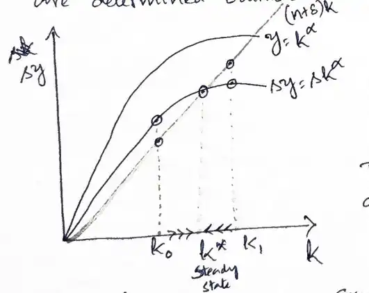
Solow diagram

Here there are two curves, the production function, using which \(sy\) is derived, which is gross investment per worker.

• \(y = k^{\alpha}\) where \(0 < \alpha < 1\) (production function in intensive form).
• \(\dot{k} = s y - (n+\delta)k\) (key equation of Solow model).

Specification

• Endogenous Variables:
  • Those variables whose values are determined within the model.
  • In this case, \(k\) and \(y\).
• Exogenous Variables (Parameters)
  • Their values are determined outside the system.
  • \(s:\) savings rate,
  • \(\delta:\) depreciation rate,
  • \(L:\) labor,
  • \(n:\) population growth rate)
• Production Function
  • \(y = k^{\alpha}\)
• Gross Investment per worker
  • \(s y = s k^{\alpha}\): Gross investment per worker.
  • It is a dampened version of \(y\) curve (translated down by factor of 's'). \(s\) is the MPS and ranges from 0 to 1.
• New investment per worker
  • \((n+\delta)k\) represents the amount of new investment Per worker required to keep the capital per worker unchanged.

Conditions for Steady State

• \(s y\) is the number of machines added per worker.
• \((n+\delta)k\) is the number of machines needed to be added per worker to keep the capital per worker unchanged.

If the number of machines added per worker (\(s y\)) is equal to the number of machines needed to be added per worker (\((n+\delta)k\)), then \(\dot{k}=0\) \(\implies\) "Steady state"

Capital Accumulation Dynamics

Mechanism

• If the number of machines added per worker is more (\(s y > (n+\delta)k\)) than the number of machines needed to be added to keep the Capital per worker unchanged, Then The capital per worker will increase (\(\dot{k}>0\)). This is called capital deepening.

• If the number of machines added per worker is less (\(s y < (n+\delta)k\)) than the needed machines to keep the capital per worker unchanged, then capital per worker will decrease (\(\dot{k}<0\)). This is called capital widening.

Interpretation of Graph

• At \(k^{*}\), the number of machines added per worker is equal to the number of machines needed to be added Per worker to keep the capital per worker unchanged (\(\dot{k}=0\)).
  • \(k^{*}\) is called Steady State and stable equilibrium.
• At \(k_{0}\) (below \(k^{*}\)), the number of machines added is more than the needed number of machines, so Capital per worker will increase till Steady state is reached.
• On the other hand, at \(k_{1}\) (above \(k^{*}\)), \(k\) is going to fall till the steady state is reached.
• It is called Stable equilibrium because We may start from any point, but finally reach the equilibrium Point.

Comparative Statics

• Comparative Statics in Solow diagram: (changing some of the parameters like saving rate, Population growth rate).

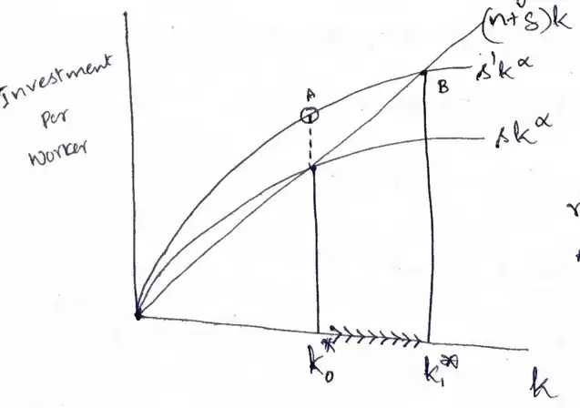
Case: Increase in savings rate (\(s\)): The initial steady state \(k_{0}^{*}\) increases to \(k_{1}^{*}\).

With an increase in saving rates, \(s'k^\alpha\), \(sy \gt (n+\delta)k\) thus, the gross investment per worker is higher than the machines that could be afforded before, thus the capital increases to ensure that \(k\) remains the same.

Hence, the initial steady state \(k_{0}^*\) increases to \(k_{1}^*\).

---

Case: Increase in Population growth rate (\(n\)): Increasing \(n\) rotates the \((n+\delta)k\) line up, decreasing the steady-state capital per worker (\(k^{*}\)).

• Steady state quantity of capital per worker is given by the condition \(\dot{k}=0\).
• We know that \(\dot{k} = s y - (n+\delta)k\).
• \(0 = s k^{\alpha} - (n+\delta)k\)
• \(s k^{\alpha} = (n+\delta)k\)
• \(\dfrac{s}{n+\delta} = \dfrac{k}{k^{\alpha}} = k^{1-\alpha}\)
• \(k^{*} = (\dfrac{s}{n+\delta})^{1/1-\alpha}\) (Steady state level of capital per worker).
• Steady state level of output per worker is:

\[y^{*} = k^{\alpha*} = [\frac{s}{n+\delta}]^{\alpha/1-\alpha}\]

Technologia (Exogenous Technological Progress, \(A\))

We looked at \(Y = F(K,L)\). To generate sustained economic growth in per capita income, we must assume technological progress (\(A\)).

Labor Augmenting / Harrod Neutral

• Production Function: \(Y = K^\alpha (AL)^{1-\alpha}\)
• Normalization (Augmented Labor): New notation \(\tilde{\boxed{\cdot}} = \dfrac{\boxed{\cdot}}{AL}\) (\(\boxed{\cdot}\) per augmented labor).
• Output per augmented labor (\(\tilde{y}\)):

\[ \dfrac{Y}{AL} = \left(\dfrac{K}{AL}\right)^\alpha \implies \tilde{y} = \tilde{k}^\alpha \]

• Steady State (\(\dot{\tilde{k}} = 0\)): \(s\tilde{y} = (n + g + \delta)\tilde{k}\) or \(s\tilde{k}^\alpha = (n + g + \delta)\tilde{k}\).

\[ \implies \dfrac{s}{(n+ g + \delta)} = \tilde{k}^{(1-\alpha)} \]

• At \(\tilde{k}^*\), it is a steady state.
• At \(\tilde{k}_{0}\), the investment being undertaken (\(s\tilde{y}\)) exceeds the amount needed to keep the capital technology ratio (CTR) constant (\((n + g + \delta)\tilde{k}\)). So the CTR will increase till the steady state is reached.

Convergence in Solow Model (Conditional)

• Convergence in Solow model:
  • Under certain circumstances, Backward Countries would tend to grow faster than rich countries, in order to close the gap between the two countries. This Phenomenon of catching up is called convergence.
• Assumptions for Convergence:
  • We have two identical countries with same Total factor Productivity growth, Labor force, and \(\delta\).
  • Among These countries, rich country has initially a higher level of capital per worker relative to the Poor country. (Consequently higher output per labor).

Here, Poor Country has lower capital labor ratio and rich Country has higher capital labor ratio. They are going to converge to steady state. However, the growth rate which Poor countries requires is more than rich countries growth rate.