Harris Torado
Assumptions
- Number of labor is constant
- Two sectors: Rural Agri & Urban Manufacturing
- Perfectly competitive markets
- Wages
- Rural = Competitive Wage
- Urban = Institutional Wage, fixed by trade unions, have minimum
- Urban employment is probabilistic
- Workers migrate if expected Urban wage \(\gt\) rural wage
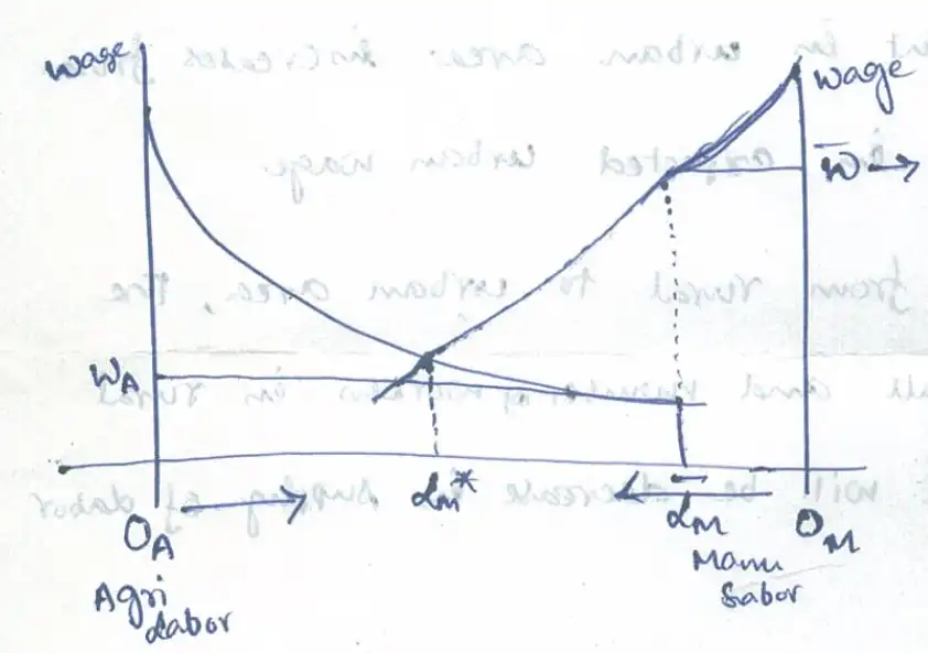
- \(O_{M}\bar{L}_{M}:\) Urban employment
- \(O_{A}L_{M}:\) Number in rural area, supply of labor
- Downward demand curve is measured by value of marginal product in agricultural sector
- \(O_{A}W_{A}:\) Agriculture sector's wage \(\lt\) Industrial wage, \(O_{M}\bar{W}\)
- \(\implies\) Migration
- \(\bar{L}:\) total labor (fixed)
- Since, the employment in urban area \(O_{M}\bar{L}_{M}\) will not increase (due to the minimum wage \(\bar{W}\)), as rural workers migrate to urban sector, there is a possibility of unemployment.
- \(p =P(\text{Getting a Job}) \lt 1\)
- Probability of getting an urban job, \(p=\dfrac{\bar{L}_{M}}{\bar{L}-L_{A}}\), where \(\bar{L}-L_{A}\) is total workers in urban sector, out of which only \(\bar{L}_{M}\) can be employed.
- As \(L_{A} \downarrow\) \(\implies\) \(\bar{L} - L_{A}\) \(\uparrow\) \(\implies\) \(P(\text{Getting a Job})\) \(\downarrow\)
- Thus, there is a decrease in the expected urban wage = \(\bar{W}P(\text{Job})\)
- As migration continues,
- In urban sector, probability to get a job decreases \(\implies\) expected wage decreases
- In the rural, since supply of rural workers decrease \(\implies\) wage starts raising
- There is a point \(O_{M}L_{M}^*\), where the Rural wage and expected urban wage will met, which is the equilibrium point at which the migration will stop.
- At the equilibrium point,
- \(L_{M}^*\bar{L}_{M}:\) Equilibrium amount of urban employment due to migration.
- \(O_{A}L^*_{M}:\) Rural workers employed.
- \(O_{M}L^*_{M}:\) Urban workers present in urban area.
- \(O_{M}\bar{L}_{M}:\) Urban workers getting job.
- Rate of urban unemployment
- \(u = \dfrac{\text{Vol of urban unemployment}}{\text{Vol of urban employment}}\)
- \(u = \dfrac{\bar{L}-L_{A}-\bar{L}_{M}}{\bar{L}_{M}}\)
- Adjust to get \(\dfrac{\bar{L}-L_{A}}{\bar{L}_{M}}-1=u\)
- Recognize that this is \(\dfrac{1}{p}-1 = u\)
- So, \(p = \dfrac{1}{1+u}\)
- Applying the equilibrium condition for migration to stop.
- "Workers migrate if expected Urban wage \(\gt\) rural wage"
- \(W_{A} = \bar{W}p\) or \(\bar{W} \dfrac{1}{1+u}\)
- Find \(u\) in terms of \(\bar{W},W_{A}\)
- We get, \(u = \dfrac{\bar{W}-W_{A}}{W_{A}}\)
\(\therefore\) The equilibrium rate of unemployment, depends on rural & urban wage differential and inversely related to rural wage.
- \(W_{A}\) \(\uparrow\) \(\implies\) \(u\) \(\downarrow\)
- \(\bar{W}\) \(\uparrow\) \(\implies\) \(u\) \(\uparrow\)
Considering Capital formation in H-T model
- Capital formation in Urban sector \(\implies\) More labor demand in urban sector \(\implies\) Fall in urban unemployment
- This happens through two forces.
\[
p \uparrow \implies \bar{W}\times p \uparrow \implies \text{Urban-rural wage gap increases}
\]
- Wage gap, \(\bar{W}p - W_{A}\) attracts more rural areas \(\implies\) urban unemployment
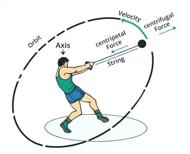
- Centrifugal force1: Downward pressure on urban employment
- Pushes labor away from the urban center
- High cost of living, unemployment, competition for jobs
- Centripetal force: Upward pressure on urban employment
- Draw labor towards the urban center
- Higher Urban wages, perceived opportunities etc
H-T model starts with full employment. But rural-urban wage gap causes urban unemployment.
-
Centrifugal force doesn't "exist" in an absolute sense, but rather is a fictitious force that appears to act on an object in a rotating reference frame because of the object's inertia – its tendency to keep moving in a straight line ↩